Section 4.4: Bases and Dimension for Vector Spaces 255
31. If 1k
v is a linear combination of the vectors 12
,,,,
k
vv v then obviously every linear
32. If the spanning set S for V is not linearly independent, then some vector in S is a
linear combination of the others. But Problem 31 says that when we remove this
33. If S is a maximal linearly independent set in V, the we see immediately that every other
34. If the minimal spanning set S for V were not linearly independent, then (by Problem
28) some vector S would be a linear combination of the others. Then the set obtained
35. Let
12
,,,
n
Svv v be a uniquely spanning set for V. Then the fact, that
36. If 12
,,,
k
aa a are scalars, then the linear combination 11 2 2 kk
cc cvv v — of the
column vectors of the matrix in Eq. (12) having the kk identity matrix as its “bottom”
kk submatrix — is a vector of the form
12
,, ,, , , ,
** * k
aa a. Hence this linear
256 Chapter 4: Vector Spaces
SECTION 4.5
ROW AND COLUMN SPACES
Conventional wisdom (at a certain level) has it that a homogeneous linear system Ax 0 of m
equations in nm unknowns ought to have nm independent solutions. In Section 4.5 of the
In each of Problems 1–12 we give the reduced echelon form E of the matrix A, a basis for the
row space of A, and a basis for the column space of A.
1.
1011
01 4
00 0
E
Row basis: The first and second row vectors of E.
Column basis: The first and second column vectors of A.
3.
1015
0113
0000
E
Row basis: The first and second row vectors of E.
Column basis: The first and second column vectors of A.
Section 4.5: Row and Column Spaces 257
5.
10 20
01 3 0
00 0 1
E
Row basis: The three row vectors of E.
Column basis: The first, second, and fourth column vectors of A.
7.
10 34
01 2 3
00 0 0
00 0 0
E
Row basis: The first two row vectors of E.
Column basis: The first two column vectors of A.
258 Chapter 4: Vector Spaces
10.
10100
01101
00011
00000
E
Row basis: The first three row vectors of E.
Column basis: The first, second, and fourth column vectors of A.
12. E is the same reduced echelon matrix as in Problem 11.
Row basis: The first three row vectors of E.
Column basis: The first, second, and fifth column vectors of A.
In each of Problems 13–16 we give the reduced echelon form E of the matrix having the given
vectors 12
,,vv as its column vectors.
Section 4.5: Row and Column Spaces 259
15.
1020
01 10
00 0 1
0000
E
Linearly independent: 12 4
,,andvv v
In each of Problems 17–20 the matrix E is the reduced echelon matrix of the matrix
11
.
kn
Av ve e
18.
12
55
3
1
55
10 0
01 0
0001 2
E
Basis vectors: 122
,,vve
260 Chapter 4: Vector Spaces
In each of Problems 21–24 the matrix E is the reduced echelon form of the transpose T
A of
the coefficient matrix .A
21.
102
011
000
E
The first and second equations are irredundant.
24.
10120
01210
00001
E
The first, second, and fifth equations are irredundant.
Section 4.5: Row and Column Spaces 261
26. The rank of the nn matrix A is n if and only if its column vectors are linearly
27. The rank of the 35 matrix A is 3, so its column vectors 11 5
,, ,aa a span 3.R
28. The rank of the 53 matrix A is 3, so its three column vectors 113
,,aaa are linearly
29. The rank of the mn matrix A is at most ,mn and therefore is less than the number
n of its column vectors. Hence the column vectors 11
,, ,
n
aa a of A are linearly
30. The rank of the mn matrix A is at most ,nm and therefore is less than the number
m of its row vectors. Hence the dimension of the column space of A is less than m, so
31. The rank of the mn matrix A is m if and only if A has m linearly independent
column vectors — in which case these m linearly independent column vectors constitute
a basis for .
m
R Hence the rank of A is m if and only if its column vectors
n
32. The rank of the mn matrix A is n if and only if the n column vectors 11
,, ,
n
aa a
of A are linearly independent — in which a vector b in m
R can be expressed in at
262 Chapter 4: Vector Spaces
33. Suppose that some linear combination of the k pivot column vectors 11
,,,
k
pp p in (8)
equals the zero vector. Denote by 11
,, ,
k
cc c the coefficients in this linear
combination. Then the first k scalar components of the equation
12 0.
k
34. If no row interchanges are involved, then (for any k) the space spanned by the first k row
vectors of A is never changed in the process of reducing A to the echelon matrix E;
35. Look at the r row vectors of the matrix A that are determined by its largest nonsingular
rr submatrix. Then Theorem 3 in Section 4.3 says that these r row vectors are
linearly independent, whereas any 1r row vectors of A are linearly dependent.
SECTION 4.6
ORTHOGONAL VECTORS IN Rn
The generalization in this section, of the dot product to vectors in ,
n
R enables us to flesh out the
algebra of vectors in n
R with the Euclidean geometry of angles and distance. We can now refer to
the vector space n
R (provided with the dot product) as n-dimensional Euclidean space.
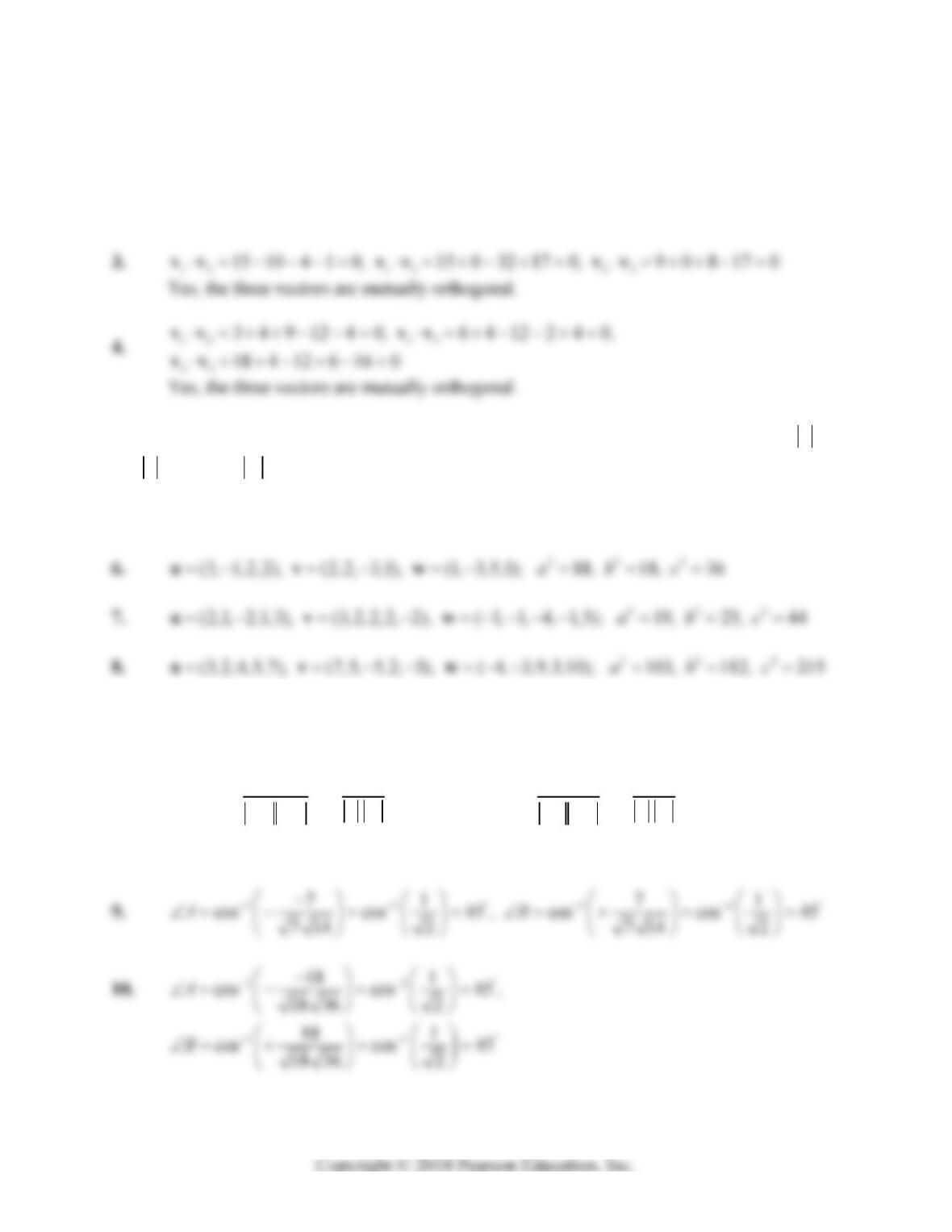
1. 12(2)(3) (1)( 6) (2)(1) (1)( 2) 6 6 2 2 0 vv
Section 4.6: Orthogonal Vectors in Rn 263
2. 12(3)(6) ( 2)(3) (3)(4) ( 4)(6) 18 6 12 24 0 vv
13(3)(17) ( 2)( 12) (3)( 21) ( 4)(3) 51 24 63 12 0 vv
23
(6)(17) (3)( 12) (4)( 21) (6)(3) 102 36 84 18 0 vv
Yes, the three vectors are mutually orthogonal.
In each of Problems 5–8 we write , , and .CB CA AB uv w
Then we calculate ,au
,bv and cw so as to verify that 22 2
.abc
5. 222
(1,1,2, 1), (1, 1,1,2), (0,2,1, 3); 7, 7, 14abc uvw
The computations in Problems 5–8 show that in each triangle ABC the angle at C is a right
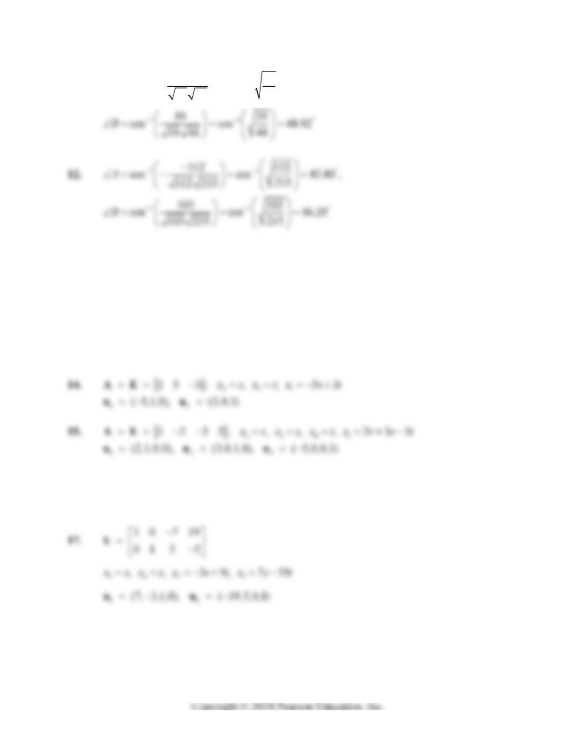
angle. The angles at the vertices A and B are then determined by the relations
cos and cos .
AB AC BA BC
AB
AB AC BA BC
vw uw
vw uw
The fact that 90AB
then serves as a check on our numerical computations.
264 Chapter 4: Vector Spaces
11. 11
25 25
cos cos 41.08 ,
44
25 44
A
In each of Problems 13–22, we denote by A the matrix having the given vectors as its row
vectors, and by E the reduced echelon form of A. From E we find the general solution of the
homogeneous system Ax 0 in terms of parameters ,, .st We then get basis vectors
12
,,uu for the orthogonal complement V by setting each parameter in turn equal to 1 (and
the others then equal to 0).
13.
231
123; , , 23
x
sx tx s t AE
12
(2,1,0), ( 3,0,1)uu
x
x
16.
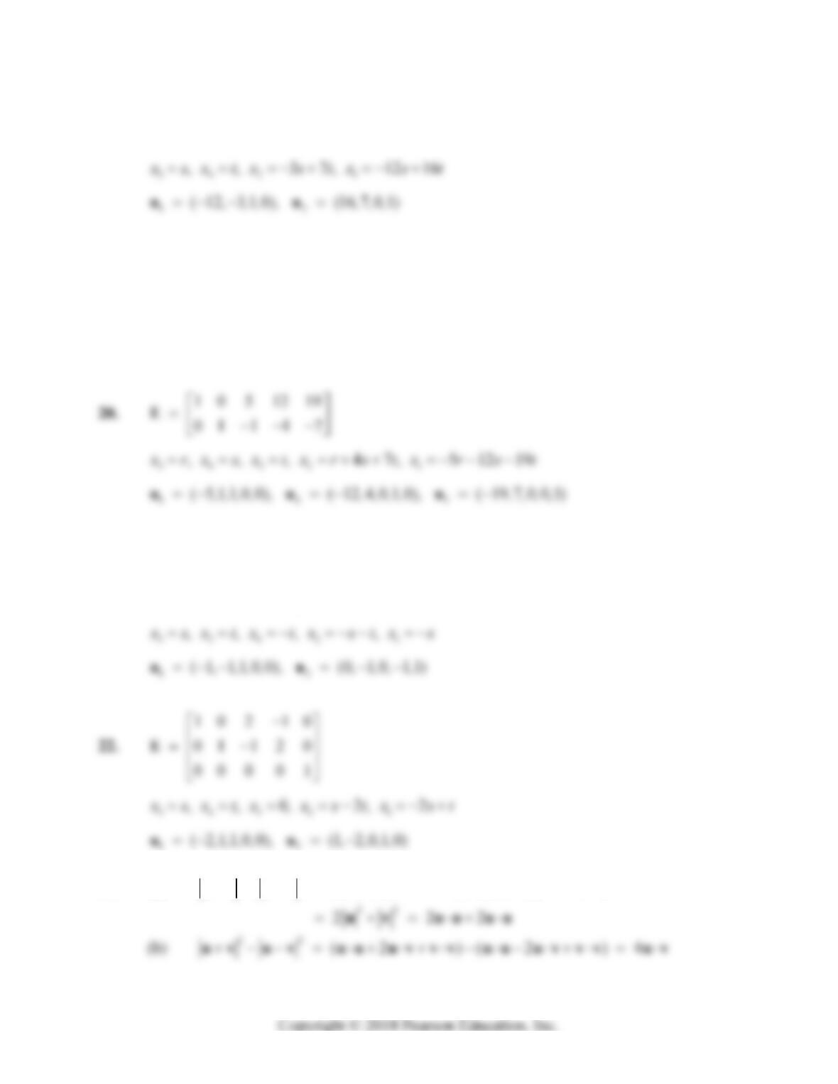
2341
17 6 9; , , , 7 6 9
x
rx sx tx r s t AE
123
( 7,1,0,0), (6,0,1,0), (9,0,0,1) uuu
x
Section 4.6: Orthogonal Vectors in Rn 265
18.
1 0 12 16
01 3 7
E
x
19. 1013 411
01 4 3 4
E
3452 1
, , , 434, 13411
x
rx sx tx r s tx r s t
123
( 13, 4,1, 0, 0), (4, 3, 0,1, 0), ( 11, 4, 0, 0,1) uuu
x
21.
10100
01101
00011
E
x
x
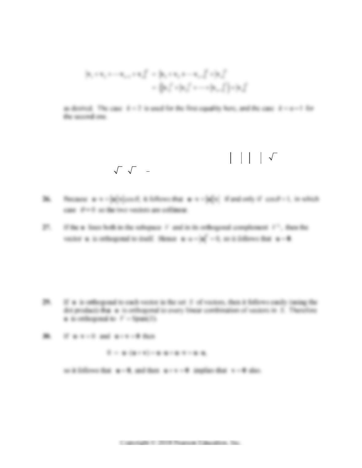
23. (a) 22
(2 )(2 ) u v u v uu uv vv uu uv vv
266 Chapter 4: Vector Spaces
24. Equation (15) in the text says that the given formula holds for 2k vectors. Assume
inductively that it holds for 1kn vectors. Then
25. Suppose, for instance, that 13
(1,0,0,0,0), (0,0,1,0,0),AB ee and
5
5(0,0,0,0,1) in .CeR
Then 31
( 1,0,1,0,0)AB ee
and
51
(0,0,1,0,0, 1).AC ee
Then 1AB AC
while 2.AB AC
It follows
that 1
2
cos 1/( 2)( 2) , so 60 .AA Similarly, 60 ,BC so we see
that ABC is an equilateral triangle.
28. If W is the orthogonal complement of V, then every vector in V is orthogonal to every
vector in W. Hence V is contained in .W But it follows from Equation (18) in this
section that the two subspaces V and W have the same dimension. Because one
contains the other, they must therefore be the same subspace, so WV
as desired.
31. We want to show that any linear combination of vectors 12
,,,
p
uu u of vectors in S is
orthogonal to every linear combination of vectors 12
,,,
q
vv v in T. But if each i
u is
orthogonal to each ,
j
v so 0,
ij
uv then it follows that
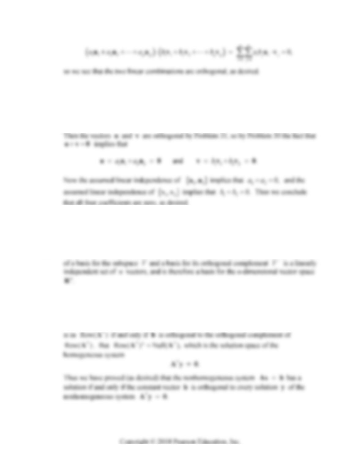
Section 4.6: Orthogonal Vectors in Rn 267
32. Suppose that the linear combination 11 2 2 11 2 2 ,aa bbuuvv0 and we want to deduce
that all four coefficients 1212
,,,aabb must necessarily be zero. For this purpose, write
11 2 2
aauuu and 11 2 2
.bbvvv
33. This is the same as Problem 32, except with
11 2 2 kk
aa a uu u u and 11 2 2 .
mm
bb bvvv v
34. It follows immediately from Problem 33 and from Equation (18) in the text that the union
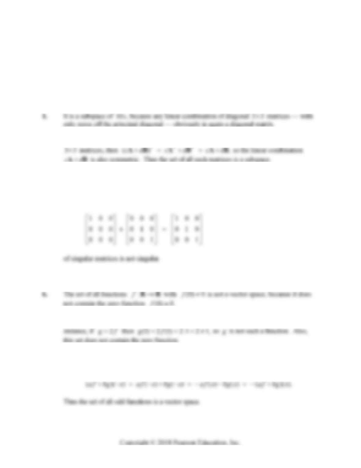
35. This is one of the fundamental theorems of linear algebra. The nonhomogeneous system
Ax b
is consistent if and only if the vector b is in the subspace Col( ) Row( ).
T
AA But b
268 Chapter 4: Vector Spaces
SECTION 4.7
GENERAL VECTOR SPACES
In each of Problems 1–12, a certain subset of a vector space is described. This subset is a subspace
of the vector space if and only if it is closed under the formation of linear combinations of its
elements. Recall also that every subspace of a vector space must contain the zero vector.
2. The square matrix A is symmetric if and only if AT = A. If A and B are symmetric
3. The set of all nonsingular 33 matrices does not contain the zero matrix, so it is not a
subspace.
4. The set of all singular 33 matrices is not a subspace, because the sum
5. The set of all functions :fRR with (0) 0f is a vector space, because if
(0) (0) 0fg then ( )(0) (0) (0) 0 0 0.af bg af bg a b
7. The set of all functions :fRR with (0) 0 and (1) 1ff is not a vector space. For
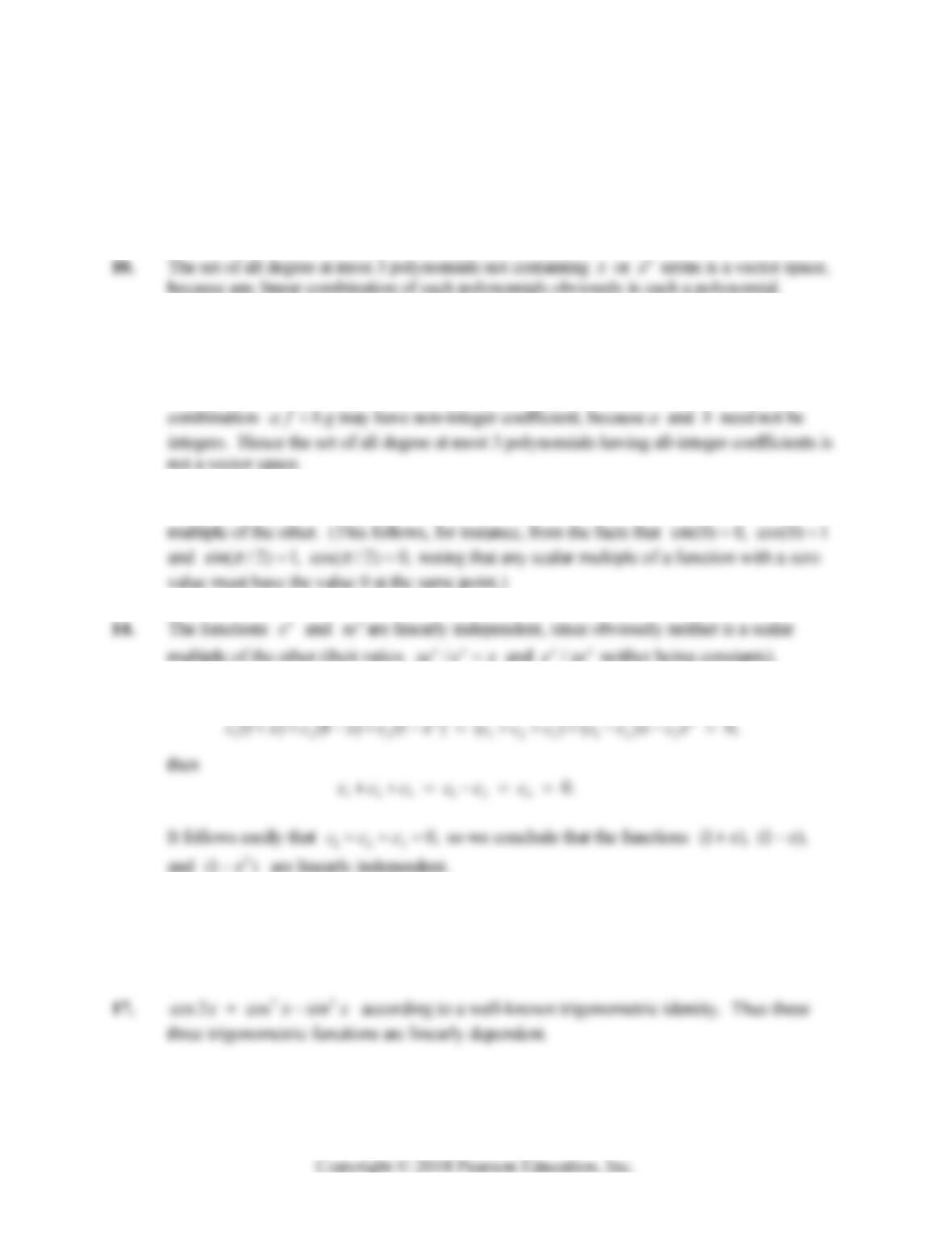
8. A function :fRR such that ( ) ( )
f
xfx is called an odd function. Any linear
combination af bg of odd functions is again odd, because
Section 4.7: General Vector Spaces 269
For Problems 9–12, let us call a polynomial of the form 23
01 2 3
aaxaxax a “degree at most 3”
polynomial.
9. The set of all degree at most 3 polynomials with nonzero leading coefficient 30a is not a
vector space, because it does not contain the zero polynomial (with all coefficients zero).
11. The set of all degree at most 3 polynomials with coefficient sum zero is a vector space,
because any linear combination of such polynomials obviously is such a polynomial.
12. If the degree at most 3 polynomials f and g have all-integer coefficients, the linear
13. The functions sin and cos
x
x are linearly independent, because neither is a scalar
x
15. If
22
x
and
x
16. 22
(1)(1 ) (1)( ) (1)(1 ) 0,xxx x so the three given polynomials are linearly
dependent.
x
270 Chapter 4: Vector Spaces
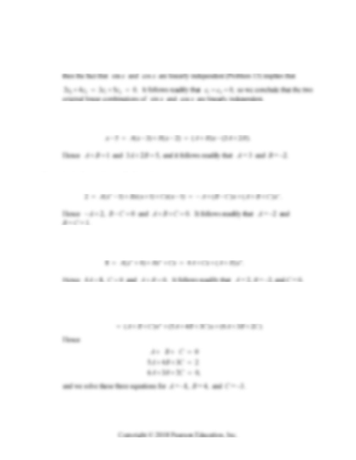
18. If
12 1212
(2cos 3sin ) (4cos 5sin ) (2 4 )cos (3 5 )sin 0cxxcxxccxccx
19. Multiplication by ( 2)( 3)xx yields
20. Multiplication by 2
(1)xx yields
21. Multiplication by 2
(4)xx yields
22. Multiplication by (1)(2)(3)xxx yields
2
2 (2)(3) (1)(3) (1)(2)
xAx x Bx x Cx x
Section 4.7: General Vector Spaces 271
23. If ( ) 0yx
then
() () (0) ,
y x y x dx dx A
24. If (4) () 0yx then
y
y
(4)
() () (0) ,
y x y x dx dx A
25. If ( )
y
x is any solution of the second-order differential equation 5 0yy
and
() (),vx y x
then ( )vx is a solution of the first-order differential equation ( ) 5 ( )vx vx
with the familiar exponential solution 5
() .
x
vx Ce Therefore
26. If ( )
y
x is any solution of the second-order differential equation 10 0yy
and
() (),vx y x
then ( )vx is a solution of the first-order differential equation
() 10()vx vx
with the familiar exponential solution 10
() .
x
vx Ce
Therefore
272 Chapter 4: Vector Spaces
27. If we take the positive sign in Eq. (20) of the text, then we have 222
vya where
() ().vx y x
Then
It follows that
( ) sinh( ) sinh cosh cosh sinh
cosh sinh .
yx a x b a x b x b
AxBx
28. We start with the second-order differential equation 0yy
and substitute
() (),vx y x
so
(taking for illustration a positive value for the arbitrary constant C). Then
(taking the positive square root). Then
Section 4.7: General Vector Spaces 273
x
It follows that
( ) sin( ) sin cos cos sin
cos sin .
yx a x b a x b x b
AxBx
Thus the general solution of the 2nd-order differential equation 0yy
is a linear
combination of cos and sin .
x
x It follows that the solution space is 2-dimensional with
basis
cos ,sin .
x
x
29. (a) The verification in a component-wise manner that V is a vector space is the same as
the verification that Rn is a vector space, except with vectors having infinitely many
components rather than finitely many components. It boils down to the fact that a linear
combination of infinite sequences of real numbers is itself such a sequence,
30. (a) If 12 12
,and
nn n n n n n n n
x
x x y y y z ax by
for each n, then
274 Chapter 4: Vector Spaces
31. (a) If 11 1
zaib and 22 2
zaib , then direct computation shows that
11 22 11 22
11 2 2 1 1 2 2
11 2 2 1 1 2 2
()()() .
ca ca cb ba
Tcz cz cTz cTz cb ba ca c a
(b) If zaib then
22
11 .
abi abi
zabiabiab