4.116
b The coefficient of determination is .0505, which indicates that only 5.05% of the variation in incomes is explained
by the variation in heights.
4.117
y = 0.6041x + 17.933
R² = 0.0505
40
50
60
70
80
90
Income
y = 19.059x + 1087.7
R² = 0.0779
2000.00
2500.00
3000.00
4.118a
4.119 B.A.
B.Sc.
y = 0.07x + 103.44
R² = 0.5201
250
300
350
400
40
60
80
15
20
B.B.A.
Other
Using the same class limits the histograms provide more detail than do the box plots.
4.120 Private course
20
30
40
20
30
40
30
40
50
Public course
4.121
a
=x
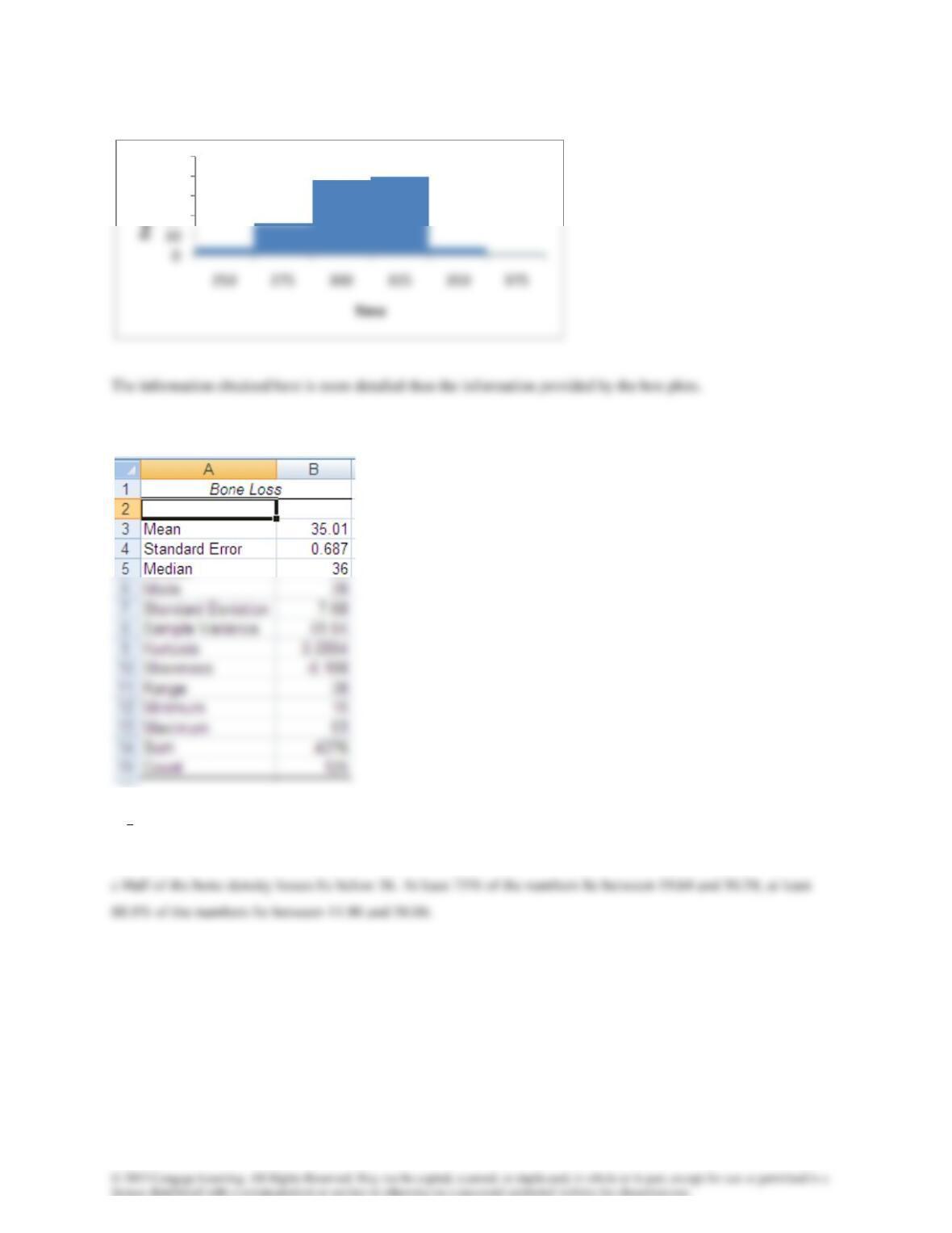
35.01, median = 36
b s = 7.68
20
30
40
50
4.122
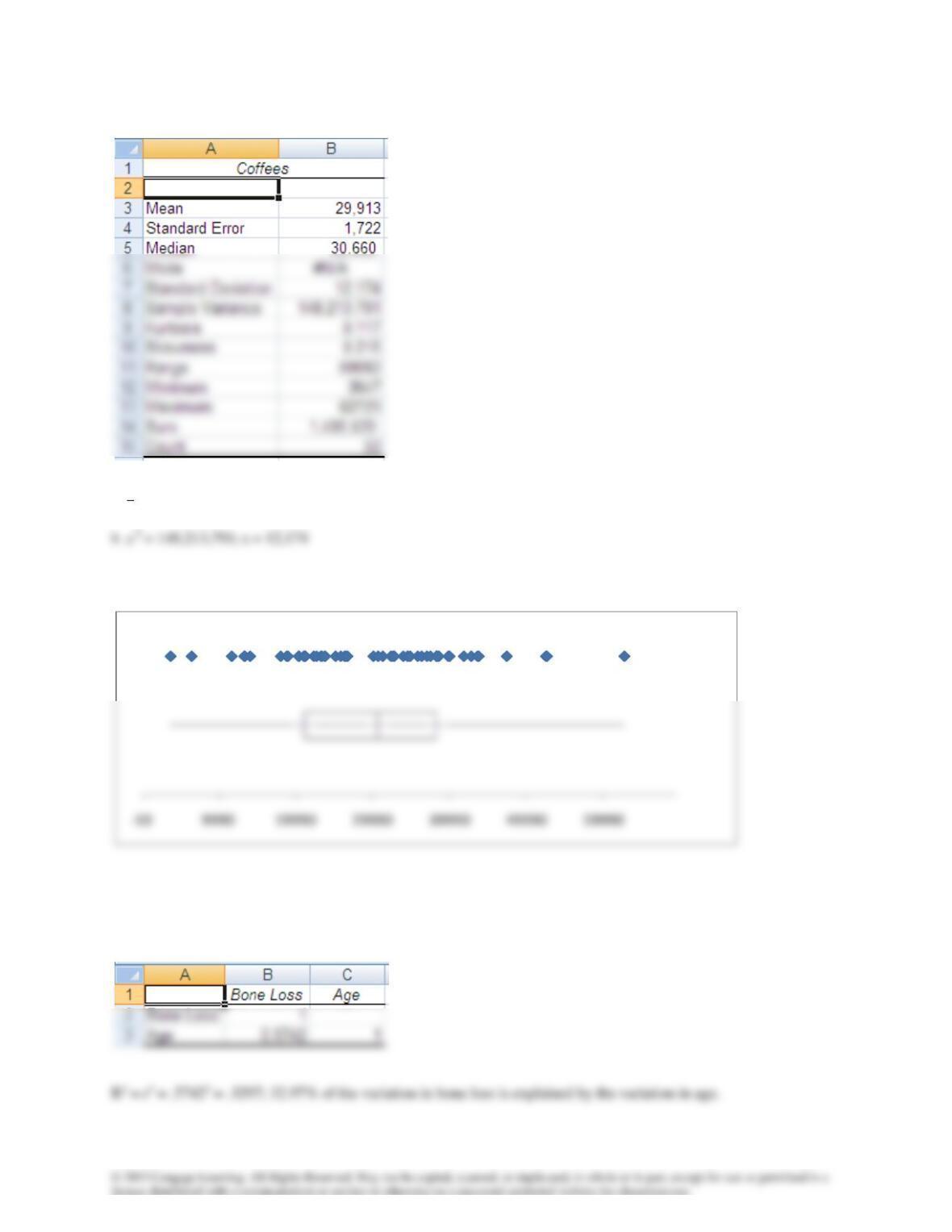
a
x
= 29,913, median = 30,660
c
d The number of coffees sold varies considerably.
4.123
4.124 a & b
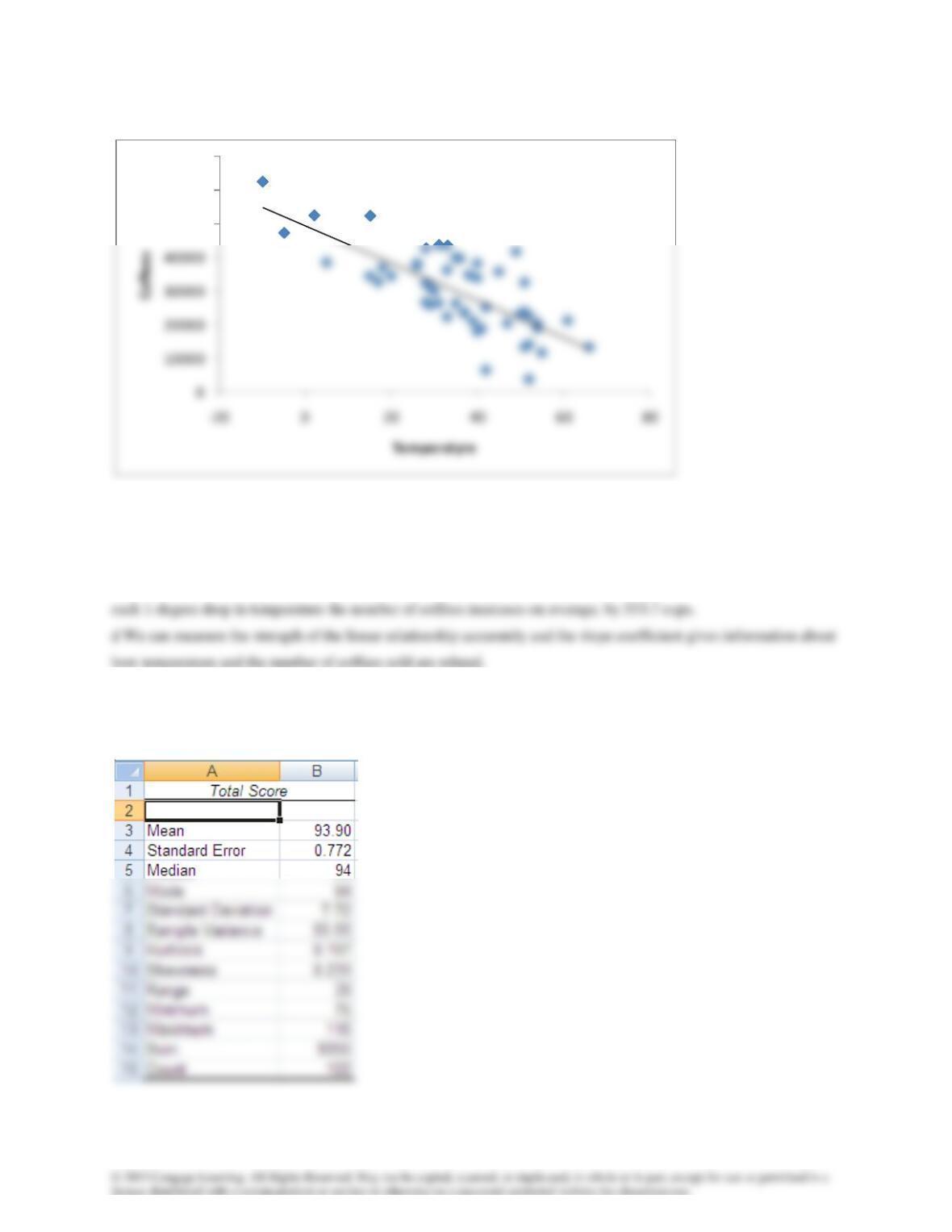
R2 = .5489 and the least squares line is
y
ˆ
= 49,337 – 553.7x
c 54.8% of the variation in the number of coffees sold is explained by the variation in temperature. For each
additional degree of temperature the number of coffees sold decreases on average by 554 cups. Alternatively for
4.125a mean, median, and standard deviation
b
y = -553.7x + 49337
R² = 0.5489
50000
60000
70000
x
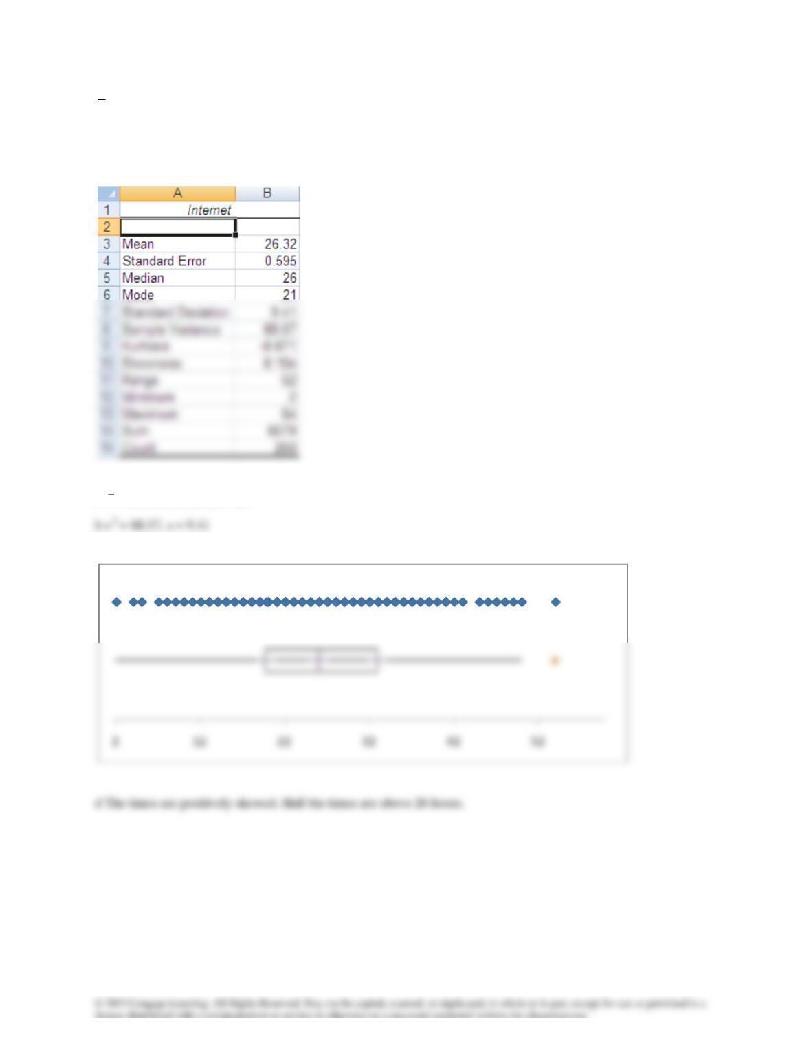
= 93.90, s = 7.72
c We hope Chris is better at statistics than he is golf.
4.126
a
x
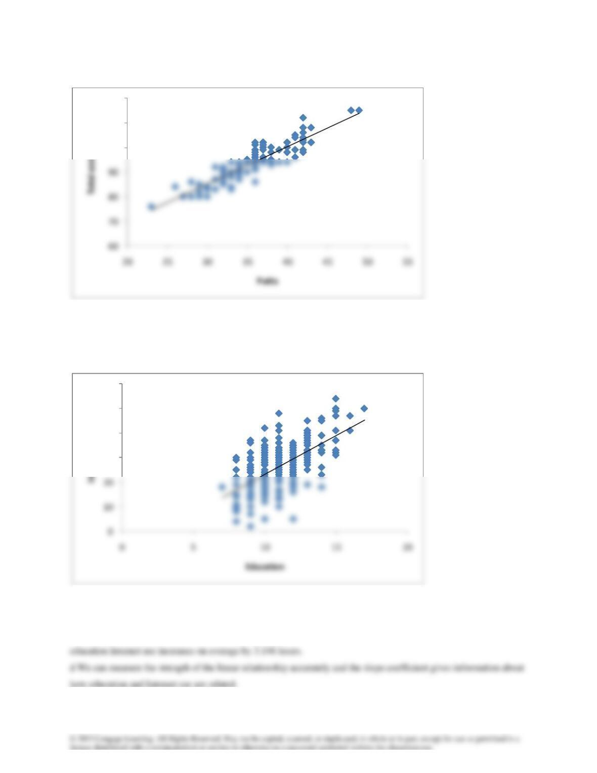
= 26.32 and median = 26
c.
4.127
80.21% of the variation in scores is explained by the variation in the number of putts.
4.128 a & b
R2 = .412 and the least squares line is
y
ˆ
= −8.2897 + 3.146x
c 41.2% of the variation in Internet use is explained by the variation in education. For each additional year of
y = 1.5176x + 39.602
R² = 0.8021
100
110
120
y = 3.146x – 8.2897
R² = 0.412
30
40
50
60
4.129
x
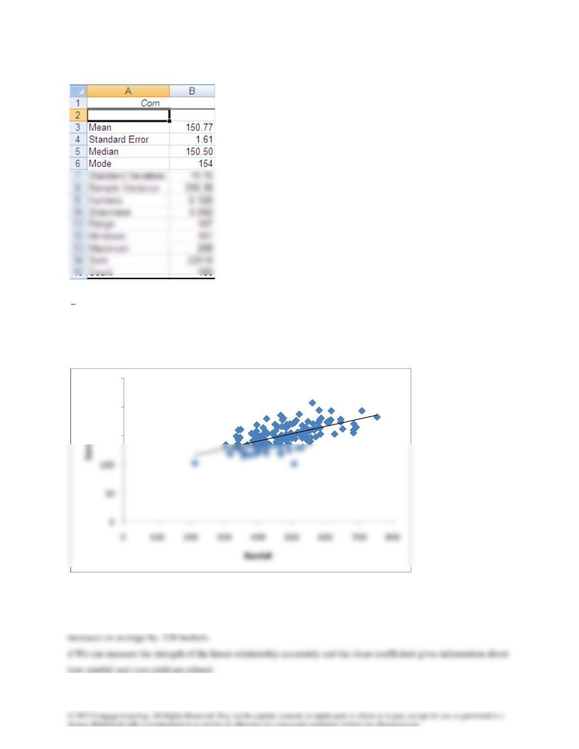
= 150.77, median = 150.50, and s = 19.76. The average crop yield is 150.77 and there is a great deal of variation
from one plot to another.
4.130a & b
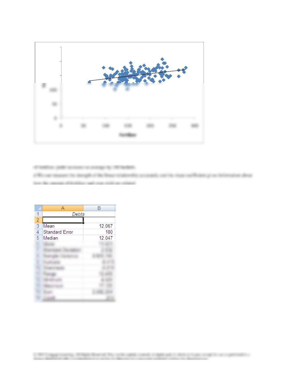
R2 = .369 and the least squares line is
y
ˆ
= 89.543 + .128 Rainfall
c 36.92% of the variation in yield is explained by the variation in rainfall. For each additional inch of rainfall yield
y = 0.128x + 89.543
R² = 0.3692
150
200
250
4.131
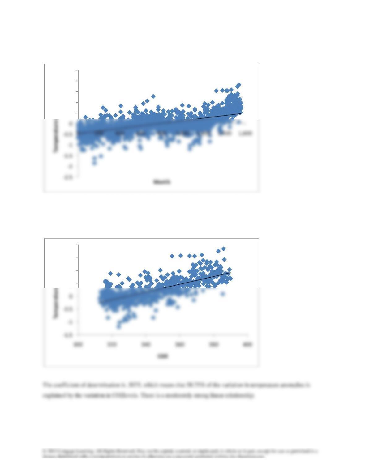
R2 = .1549 and the least squares line
y
ˆ
= 120.37 + .1802 Fertilizer
c 15.49% of the variation in yield is explained by the variation in the amount of fertilizer. For each additional unit
4.132a
b The mean debt is $12,067. Half the sample incurred debts below $12,047 and half incurred debts above. The mode
is $11,621.
y = 0.1802x + 120.37
R² = 0.1549
150
200
250
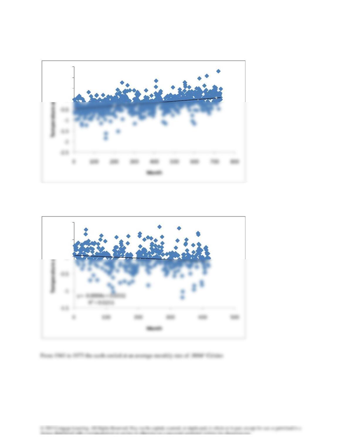
Case 4.1 a Scatter diagrams with time as the independent variable and temperature anomalies as the dependent
variable
Monthly average increase is .0006. For the 1600 month period the increase was 1600(.0006) = .96o Celsius.
Scatter diagrams with carbon dioxide levels as the independent variable and temperature anomalies as the dependent
variable
y = 0.0006x – 0.4754
R² = 0.3708
0.5
1
1.5
2
2.5
y = 0.0151x – 4.9604
R² = 0.5075
0.5
1
1.5
2
Case 4.2
1880 to 1940
From 1880 to 1940 the earth warned at an average monthly rate of .0007o Celsius.
1941 to 1975
y = 0.0007x – 0.4776
R² = 0.1919
0
0.5
1
1.5
0
0.5
1
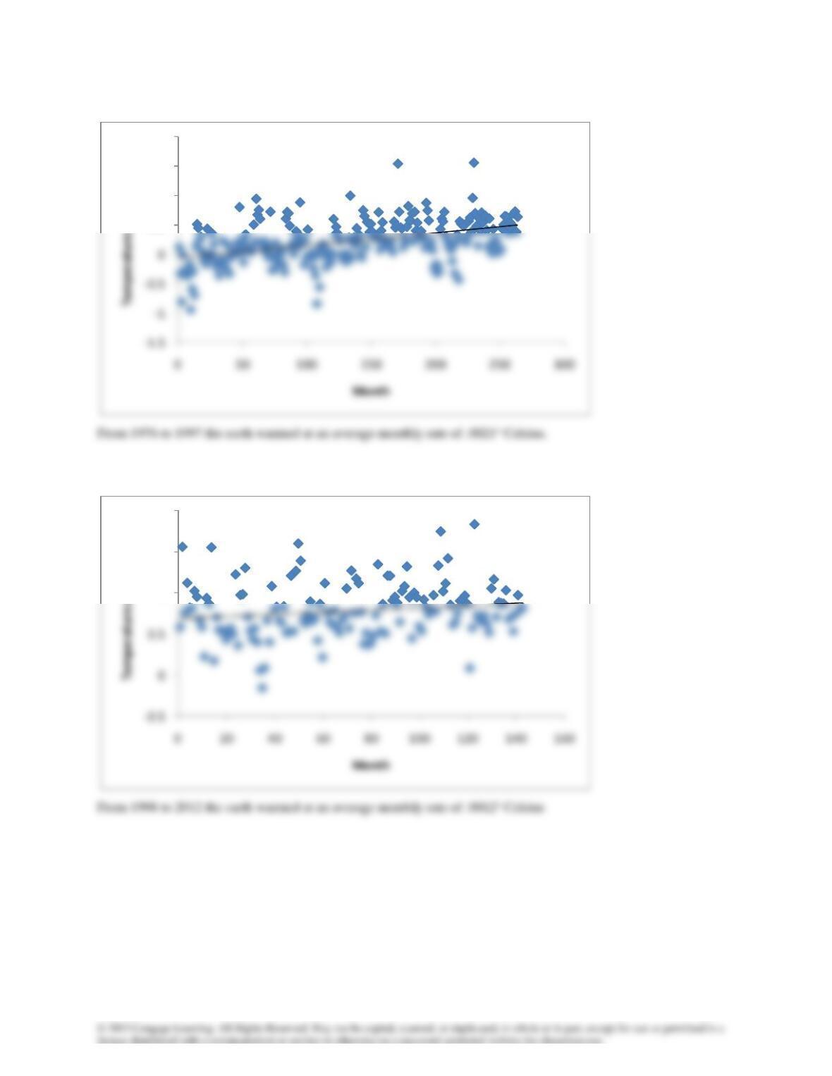
1976 to 1997
1998 to 2012
Over different periods of time the earth has warmed and cooled.
y = 0.0021x – 0.0581
R² = 0.197
0.5
1
1.5
2
y = 0.0012x + 0.6932
R² = 0.0241
1
1.5
2
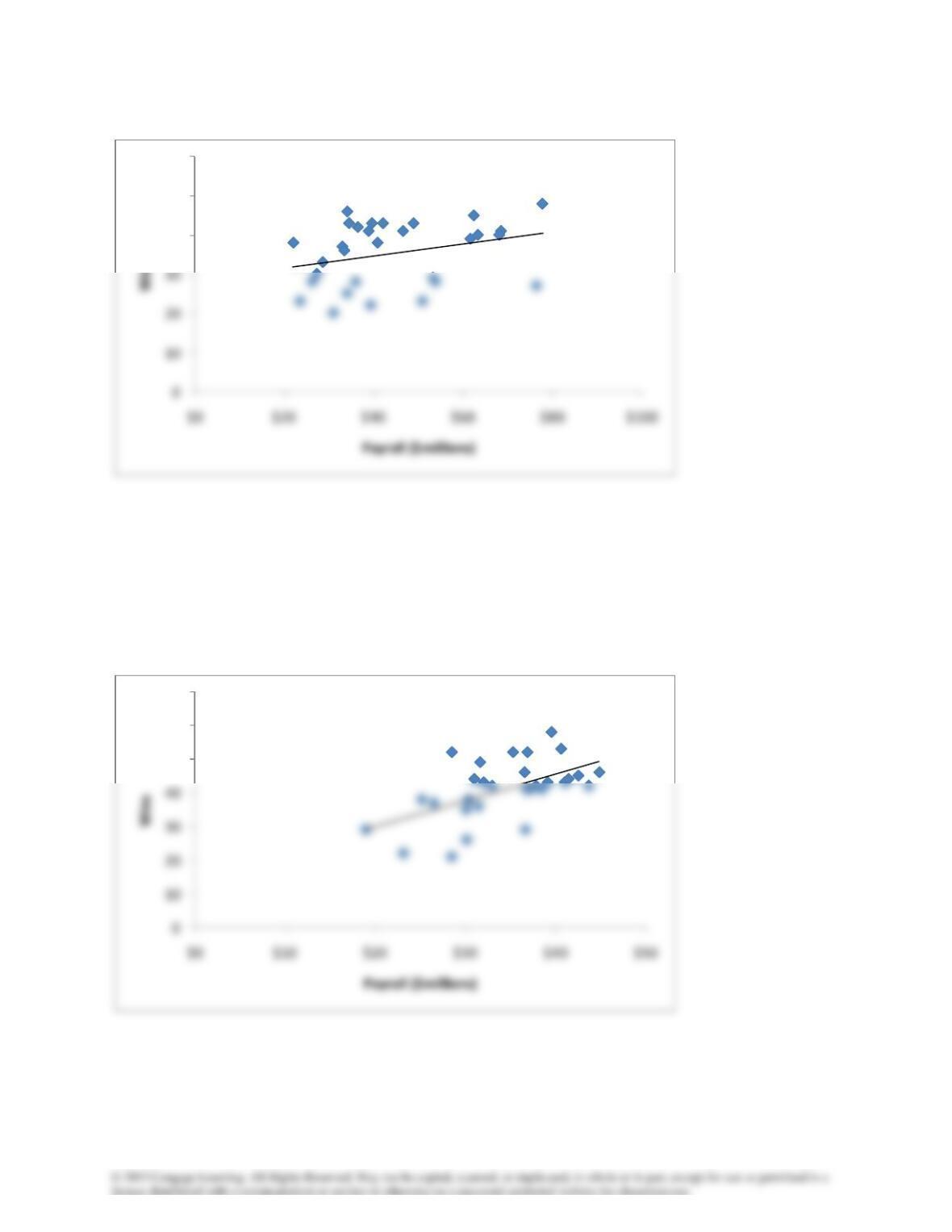
Case 4.3 2003-04 Season
The cost of winning one additional game is 1million/.1526 = $6.553 million. However, the coefficient of
determination is only .0876, which tells us that there are many other variables that determine how well a team will
do.
2005-06 Season
The cost of winning one additional game is 1million/.7795 = $1.283 million. The coefficient of determination is
.3072.
y = 0.1526x + 28.559
R² = 0.0876
40
50
60
y = 0.7795x + 14.256
R² = 0.3072
50
60
70
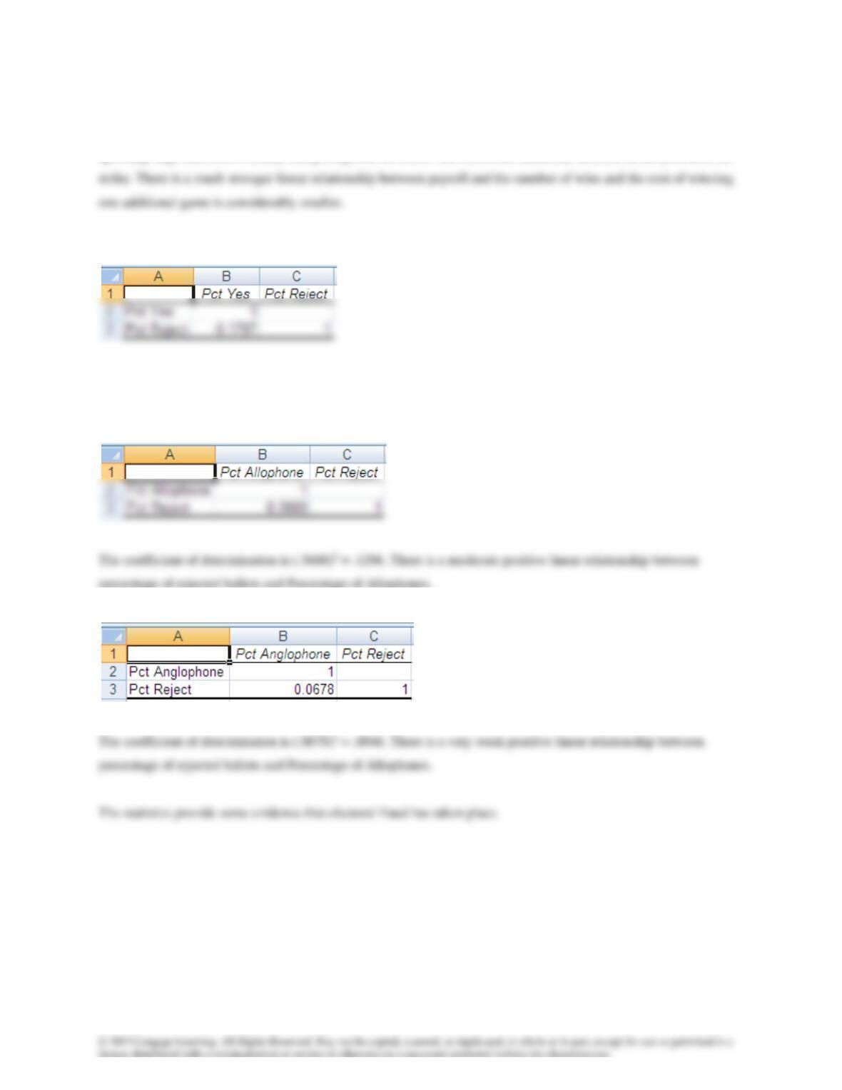
The small coefficient of determination in the year before the strike seems to indicate that team owners were
spending large amounts of money and getting little in return. The results are markedly different in the year after the
Case 4.4
The coefficient of determination is (−.1787)2 = .0319. There is a weak negative linear relationship between
percentage of rejected ballots and Percentage of “yes” votes.
percentage of rejected ballots and Percentage of Allophones.