Section 3.1: Introduction to Linear Systems 175
17. First we subtract the first equation from the second equation to get the new first equation
36 4.xyz Then subtraction of three times the new first equation from the second
18. Subtraction of the five times the first equation from the second equation gives
19. Subtraction of twice the first equation from the second equation gives 3 6 9.yz
20. First we subtract the second equation from the first equation to get the new first equation
65.xy z Then subtraction of the new first equation from the second equation
gives 5 5 25,yz and subtraction of the new first equation from the third equation
21. Subtraction of three times the first equation from the second equation gives 3 6 9.yz
32.
x
t
22. Subtraction of four times the second equation from the first equation gives 2100.yz
x
23. The initial conditions (0) 3 and (0) 8yy
yield the equations 3and2 8,AB
so
3 and 4.AB
It follows that () 3cos2 4sin2.yx x x
24. The initial conditions (0) 5 and (0) 12yy
yield the equations 5and3 12,AB
so 5 and 4.AB
It follows that ( ) 5cosh3 4sinh3 .yx x x
176 Chapter 3: Linear Systems and Matrices
x
27. The initial conditions (0) 40 and (0) 16yy
yield the equations 40 andAB
35 16AB
with solution 23, 17.AB Thus 35
( ) 23 17 .
x
x
y
xee
x
y
y
30. The initial conditions (0) 41 and (0) 164yy
yield the equations 41 andAB
47164
35
AB with solution 81, 40.AB Thus 4/3 7/5
( ) 81 40 .
xx
yx e e
31. The graph of each of these linear equations in x and y is a straight line through the
origin (0, 0) in the xy-plane. If these two lines are distinct then they intersect only at the
32. The graph of each of these linear equations in x, y, and z is a plane in xyz-space. If these
33. (a) The three lines have no common point of intersection, so the system has no
solution.
(b) The three lines have a single point of intersection, so the system has a unique
solution.
Section 3.2: Matrices and Gaussian Elimination 177
34. (a) If the three planes are parallel and distinct, then they have no common point of
intersection, so the system has no solution.
(b) If the three planes coincide, then each of the infinitely many different points
(, ,)
x
yz of this common plane provides a solution of the system.
x
x
SECTION 3.2
MATRICES AND GAUSSIAN ELIMINATION
Because the linear systems in Problems 1–10 are already in echelon form, we need only start at the
end of the list of unknowns and work backwards.
1. Starting with 32x from the third equation, the second equation gives 20,x and then
the first equation gives 11.x
x
x
x
4. If we set 3
x
t then the second equation gives 257,
x
t and next the first equation
gives 135 33 .
x
t
5. If we set 4
x
t then the third equation gives 353,
x
t next the second equation gives
x
x
x
178 Chapter 3: Linear Systems and Matrices
7. If we set 3
x
s and 4,
x
t then the second equation gives 272 7,
x
st and next
the first equation gives 138 19.
x
st
x
x
x
x
10. If we set 3
x
s and 5,
x
t then the third equation gives 45,
x
t next the second
equation gives 213 8 ,
x
st and finally the first equation gives 163 16 .
x
st
11. Begin by interchanging rows 1 and 2 of A. Then subtract twice row 1 both from row 2
and from row 3.
132 5
12. Begin by subtracting row 2 of A from row 1. Then subtract twice row 1 both from row
2 and from row 3.
12 3
16415
01 0 3; 5, 3, 2
00 1 2
xx x
E
Section 3.2: Matrices and Gaussian Elimination 179
14. Begin by interchanging rows 1 and 3 of A. Then subtract twice row 1 from row 2, and
three times row 1 from row 3.
123
1229
00 1 7; 52, , 7
0000
xtxtx
E
16. Begin by subtracting row 1 from row 2 of A. Then interchange rows 1 and 2. Next
subtract twice row 1 from row 2, and five times row 1 from row 3.
1476
01 20.
00 01
E The system has no solution.
17. 1234
433 4xxxx
18. Begin by subtracting row 3 from row 1 of A. Then subtract 3 times row 1 from row 2,
and twice row 1 from row 3.
180 Chapter 3: Linear Systems and Matrices
19. Begin by interchanging rows 1 and 2 of A. Then subtract three times row 1 from row 2,
and four times row 1 from row 3.
20. Begin by interchanging rows 1 and 2 of A. Then subtract twice row 1 from row 2, and
five times row 1 from row 3.
22. Begin by subtracting row 4 from row 1. Then subtracting twice row 1 from row 2, four
times row 1 from row 3, and three times row 1 from row 4.
12 3 4
12409
01 6121
; 3,2,4,1
00 104
00 01 1
xx x x
E
23. If we subtract twice the first row from the second row, we obtain the echelon form
Section 3.2: Matrices and Gaussian Elimination 181
24. If we subtract twice the first row from the second row, we obtain the echelon form
25. If we subtract twice the first row from the second row, we obtain the echelon form
26. If we first subtract twice the first row from the second row, then interchange the two rows,
and finally subtract 3 times the first row from the second row, then we obtain the echelon
form
27. If we first subtract twice the first row from the second row, then subtract 4 times the first
row from the third row, and finally subtract the second row from the third row , we obtain
the echelon form
28. If we first interchange rows 1 and 2, then subtract twice the first row from the second row,
next subtract 7 times the first row from the third row, and finally subtract twice the second
row from the third row , we obtain the echelon form
182 Chapter 3: Linear Systems and Matrices
29. In each of parts (a)-(c), we start with a typical 2 2 matrix A and carry out two row
successive operations as indicated, observing that we wind up with the original matrix A.
(a)
(1/ ) 2
2cR
cR
st s t st
uv cucv uv
AA
30. (a) This part is essentially obvious, because a multiple of an equation that is satisfied is
also satisfied, and the sum of two equations that are satisfied is one that is also satisfied.
(b) Let us write 112 1 2
,, ,,
nn
ABB BB A
where each matrix 1k
B is obtained
Section 3.3: Reduced Row-Echelon Matrices 183
SECTION 3.3
REDUCED ROW-ECHELON MATRICES
Each of the matrices in Problems 1-20 can be transformed to reduced echelon form without the
appearance of any fractions. The main thing is to get started right. Generally our first goal is to get
a 1 in the upper left corner of A, then clear out the rest of the first column. In each problem we
first give at least the initial steps, and then the final result E. The particular sequence of elementary
row operations used is not unique; you might find E in a quite different way.
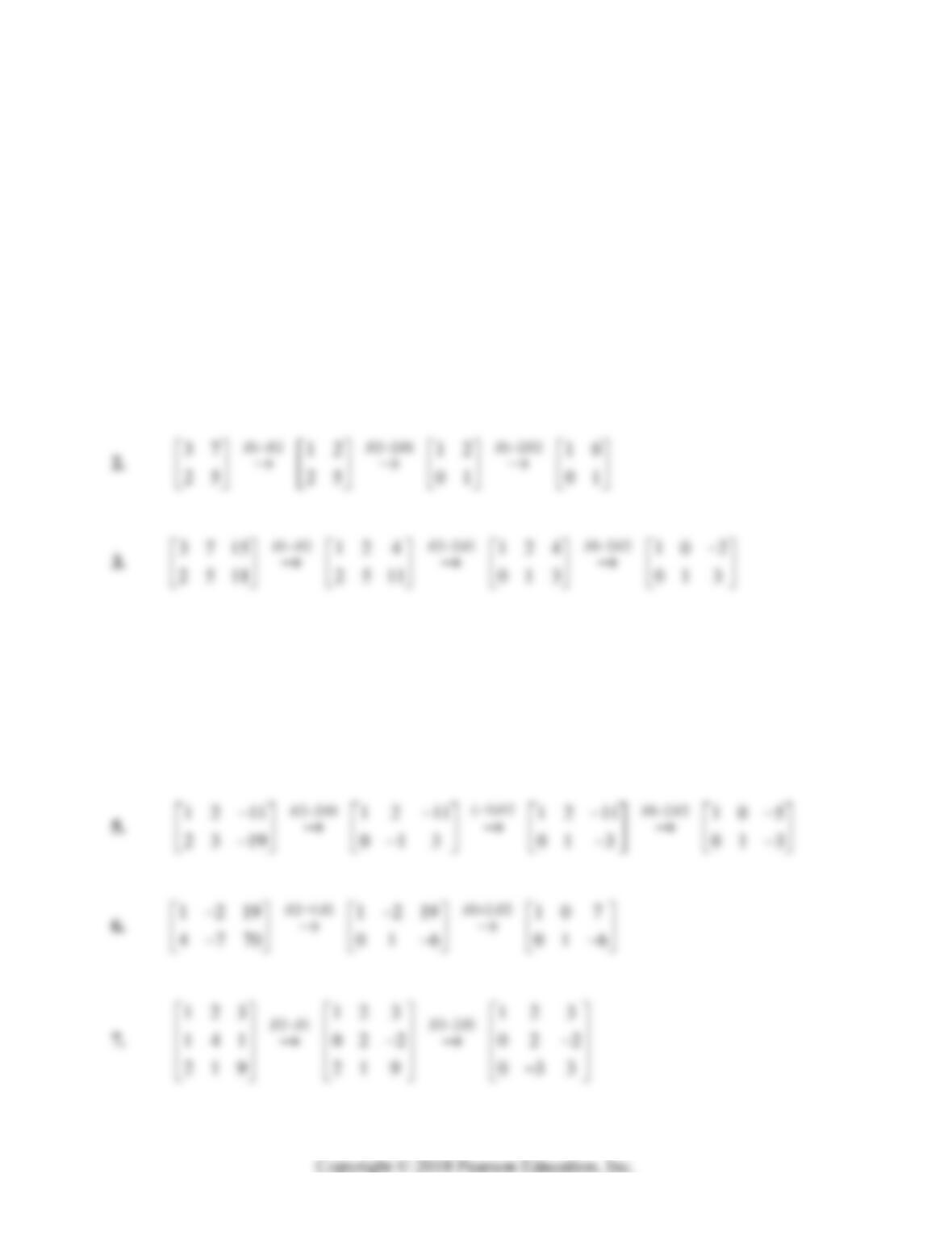
1.
231 12 2
12 12 10
37 01 01
RR RR
4.
21 12
37 1 3 7 1 112 10
52 8 2 5 9 2 5 9
RR RR
(1/29) 2 112 2
221 1 12 10 1 12 10 1 0 2
02929 01 1 011
RRR
RR
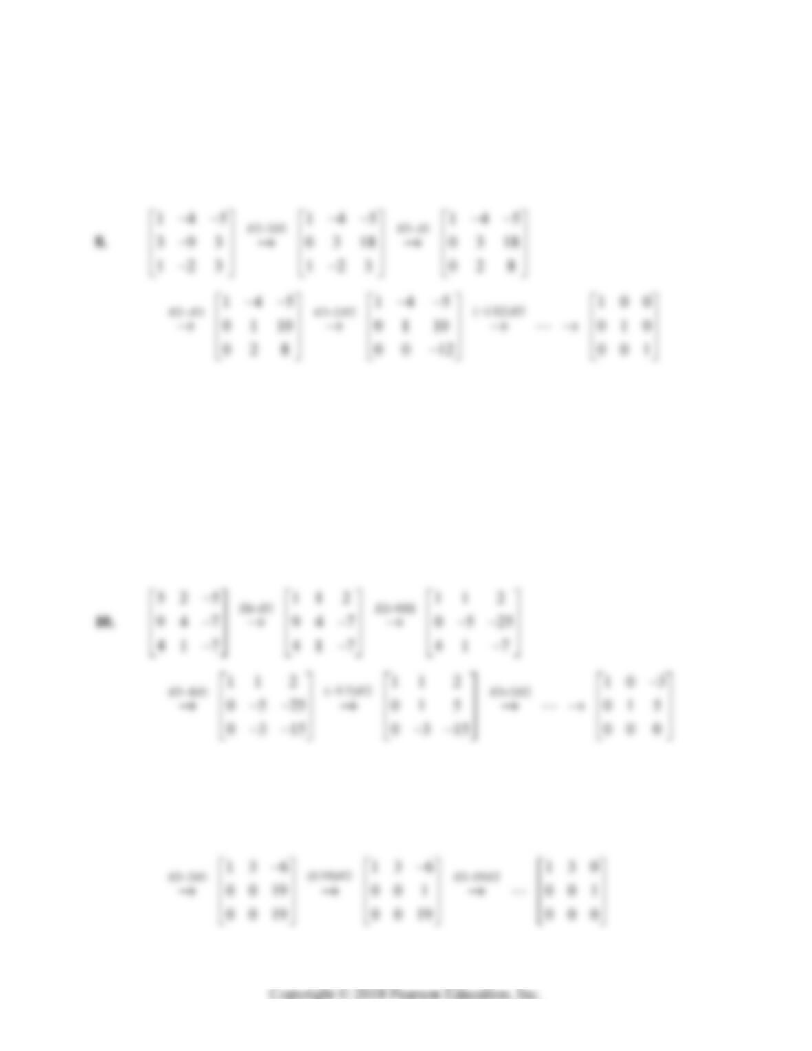
184 Chapter 3: Linear Systems and Matrices
(1/ 2) 2 33 2 12 2
12 3 123 105
01 1 01 1 01 1
033 000 000
RRR RR
9.
13 341
5218 116 1 1 6
01 4 01 4 0 1 4
4 1 12 4 1 12 0 3 12
RR R R
33 2 1 2
116 102
014 014
000 000
RR RR
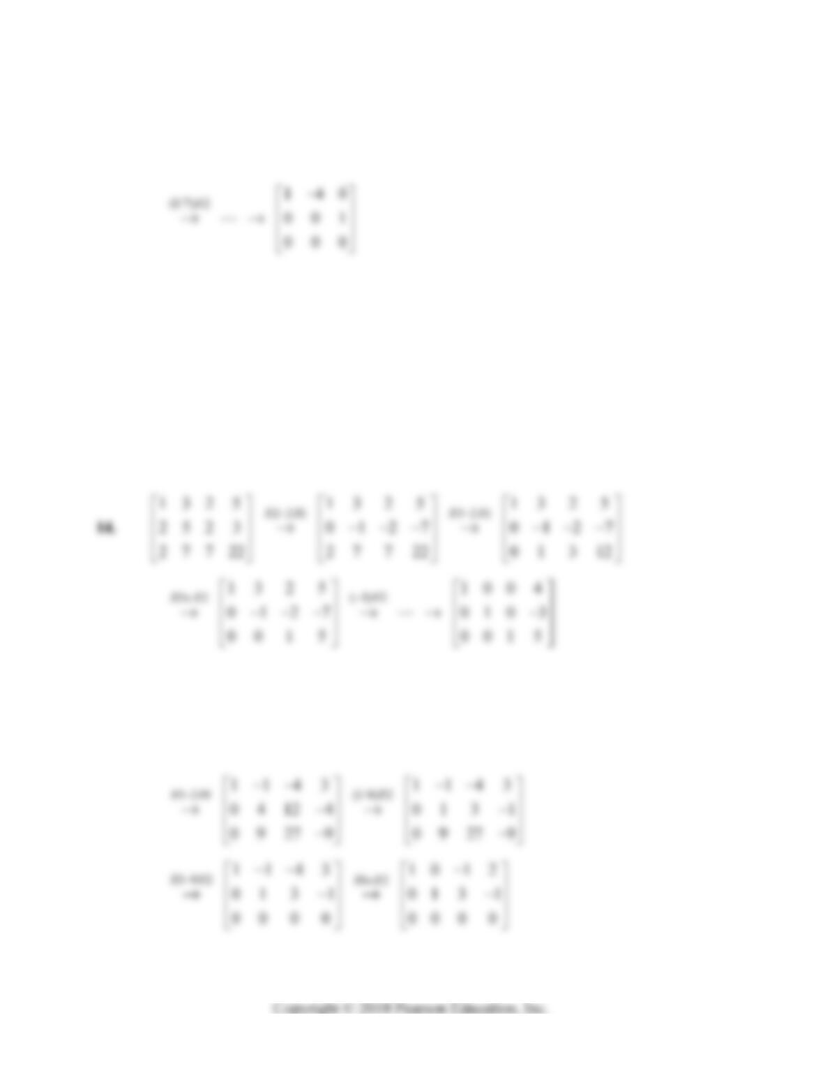
11.
(1,3) 221
39 1 13 6 13 6
26 7 26 7 0019
13 6 39 1 39 1
SWAP R R RR
Section 3.3: Reduced Row-Echelon Matrices 185
12.
23 1 32 1
142 142 142
3121 007 007
285 285 009
RR RR
13.
(1,2) 22 1
2740 1321 132 1
1321 2740 010 2
2654 2654 265 4
SWAP R R RR
22 1 13 2
132 1 100 3
010 2 010 2
001 2 001 2
RR RR
15.
(1,2) 22 1
2242 1143 1143
1143 2242 04124
2719 3 2719 3 2719 3
SWAP R R RR
186 Chapter 3: Linear Systems and Matrices
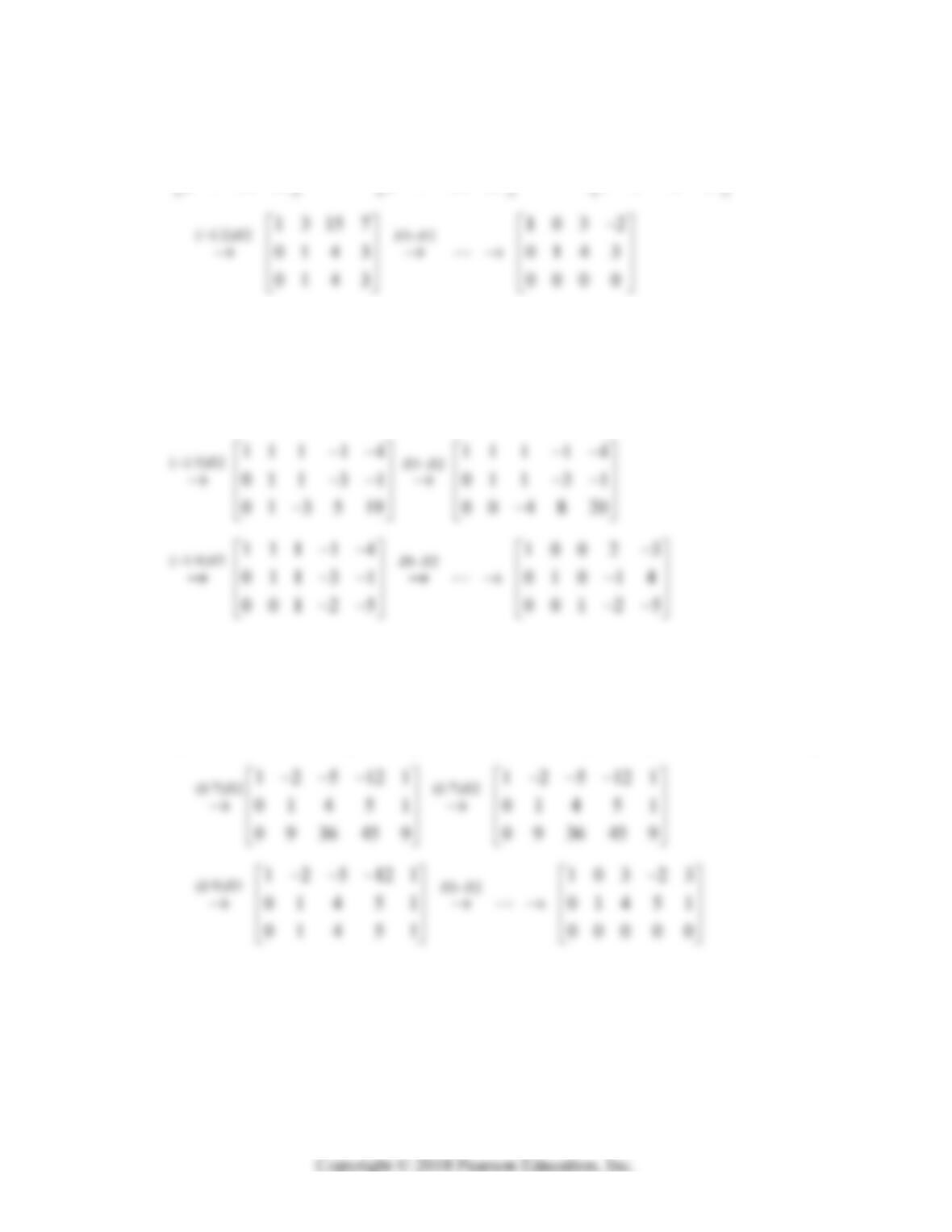
16.
22 1 32 1
1 3 15 7 1 3 15 7 1 3 15 7
24228 0286 0286
2 7 34 17 2 7 34 17 0 1 4 3
RR RR
17.
32 1
21
11 1 1 4 11 1 1 4 11 1 1 4
1228 1 03393 03393
2 3 1 3 11 2 3 1 3 11 0 1 3 5 19
RR
RR
18.
32 1
221
125121 125121 125121
2 3 18 11 9 0 7 28 35 7 0 7 28 35 7
2 5 26 21 11 2 5 26 21 11 0 9 36 45 9
RR
RR
Section 3.3: Reduced Row-Echelon Matrices 187
19.
(1,3)
2 7 10 19 13 1 0 2 1 3
13 4 8 6 13 4 8 6
10 2 1 3 27 10 1913
SWAP R R
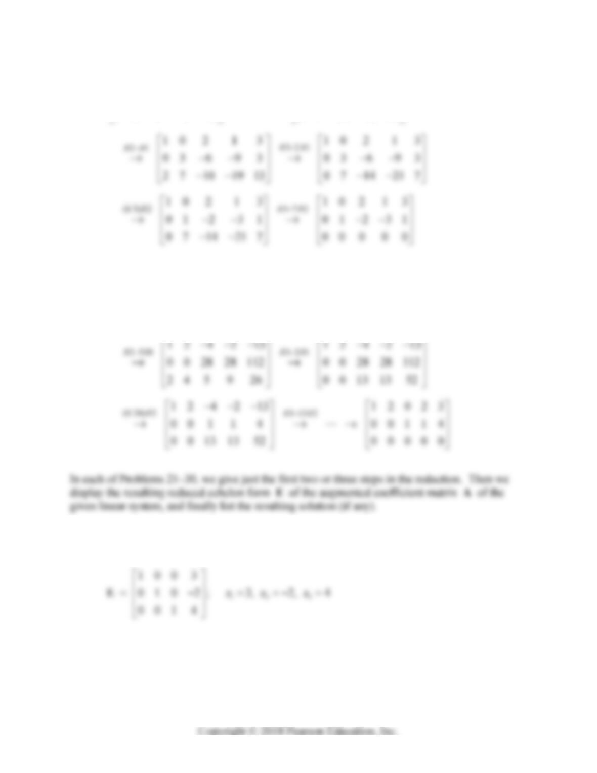
20.
13
361713 12 4213
5 10 8 18 47 5 10 8 18 47
2 4 5 9 26 2 4 5 9 26
RR
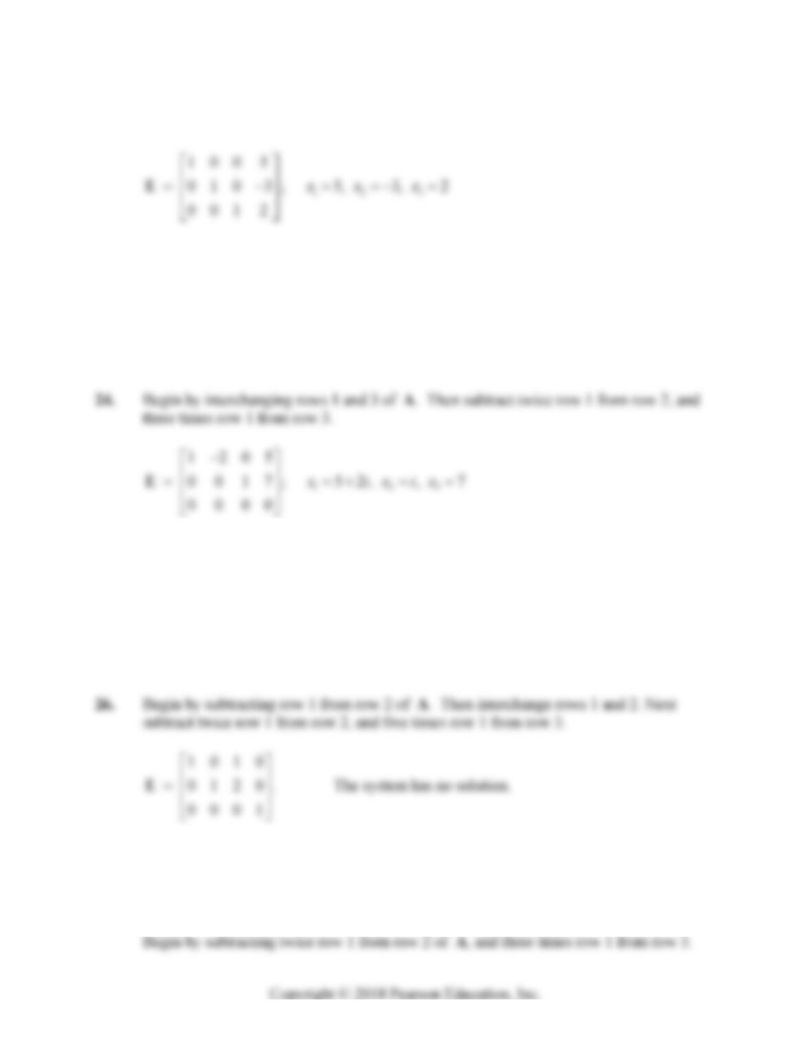
21. Begin by interchanging rows 1 and 2 of A. Then subtract twice row 1 both from row 2
and from row 3.
188 Chapter 3: Linear Systems and Matrices
22. Begin by subtracting row 2 of A from row 1. Then subtract twice row 1 both from row
2 and from row 3.
23. Begin by subtracting twice row 1 of A both from row 2 and from row 3. Then add row
2 to row 3.
123
10 314
01 2 3; 43, 32,
00 0 0
x
tx tx t
E
25. Begin by interchanging rows 1 and 2 of A. Then subtract three times row 1 from row 2,
and five times row 1 from row 3.
10 20
01 3 0.
00 0 1
E The system has no solution.
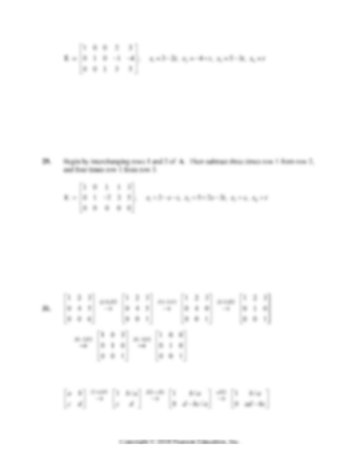
27. 1234
433 4xxxx
1234
2655 5xxxx
1234
3457xxxx
Section 3.3: Reduced Row-Echelon Matrices 189
x
28. Begin by subtracting row 3 from row 1 of A. Then subtract 3 times row 1 from row 2,
and twice row 1 from row 3.
1234
12034
00143; 423, , 34,
00000
x
stxsx txt
E
x
30. Begin by interchanging rows 1 and 2 of A. Then subtract twice row 1 from row 2, and
five times row 1 from row 3.
12 3 45
100 0 32
010 1 2 1; 23, 1 2, 22, ,
001 2 0 2
x
tx s tx sx sx t
E
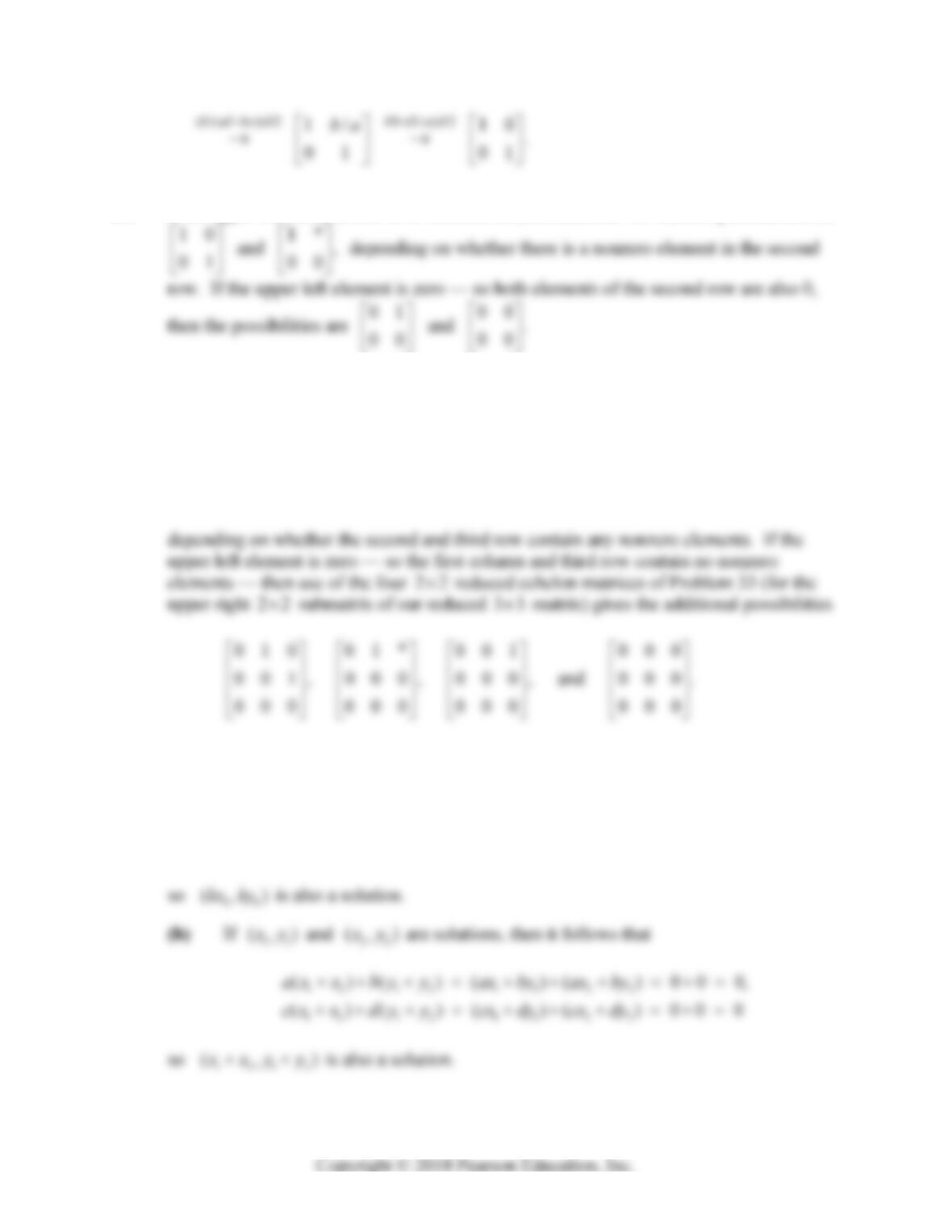
32. If 0,ad bc then not both a and b can be zero. If, for instance,
0,a
then
190 Chapter 3: Linear Systems and Matrices
33. If the upper left element of a 2 2 reduced echelon matrix is 1, then the possibilities are
34. If the upper left element of a 33 reduced echelon matrix is 1, then the possibilities are
100 10* 1*0 1**
010, 01*, 001, and 000,
001 000 000 000
35. (a) If 00
(, )
x
y is a solution, then it follows that
00 00
00 00
()() ( ) 0 0,
() () ( ) 0 0
akx bky kax by k
ckx dky kcx dy k
Section 3.3: Reduced Row-Echelon Matrices 191
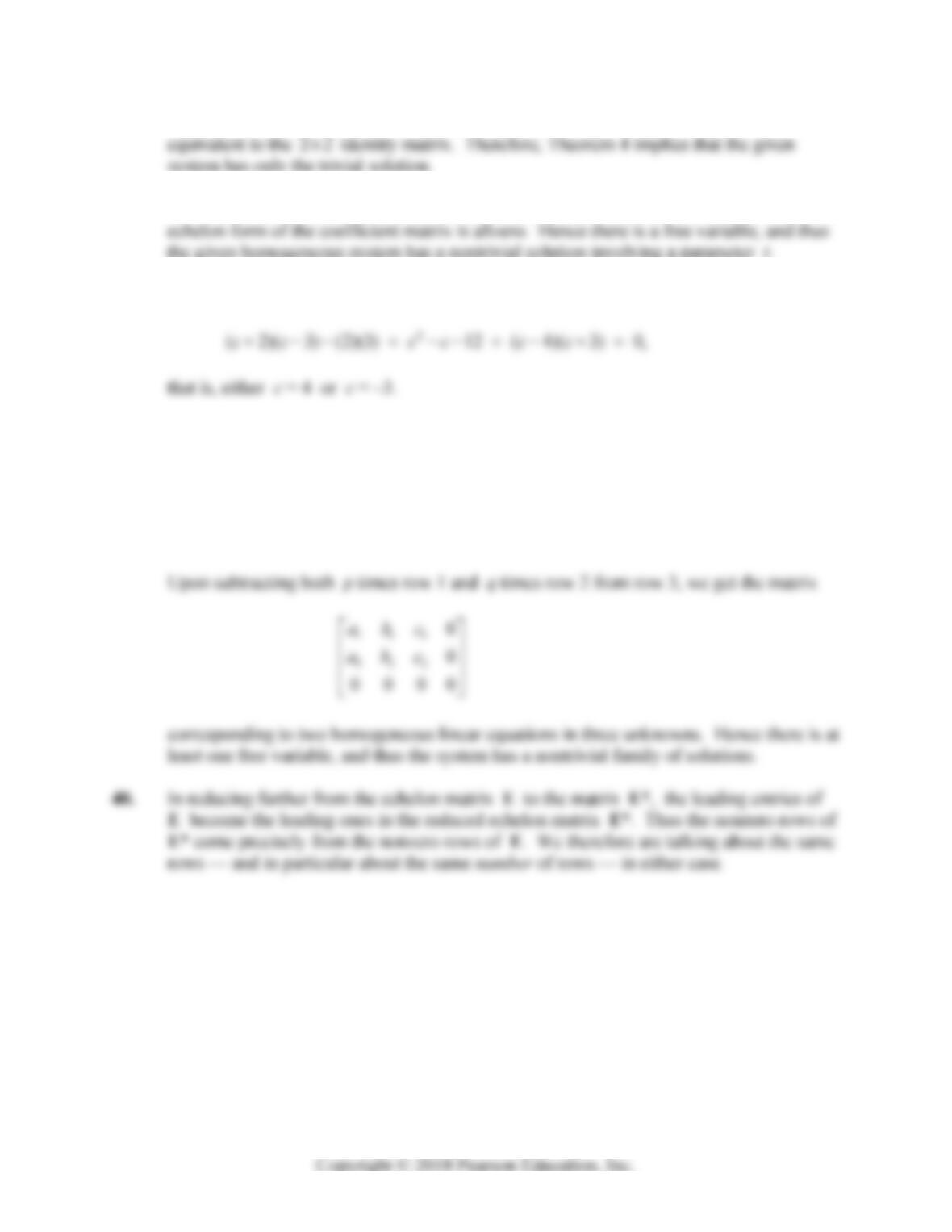
36. By Problem 32, the coefficient matrix of the given homogeneous 22 system is row-
37. If 0ad bc then, much as in Problem 32, we see that the second row of the reduced
38. By Problem 37, there is a nontrivial solution if and only if
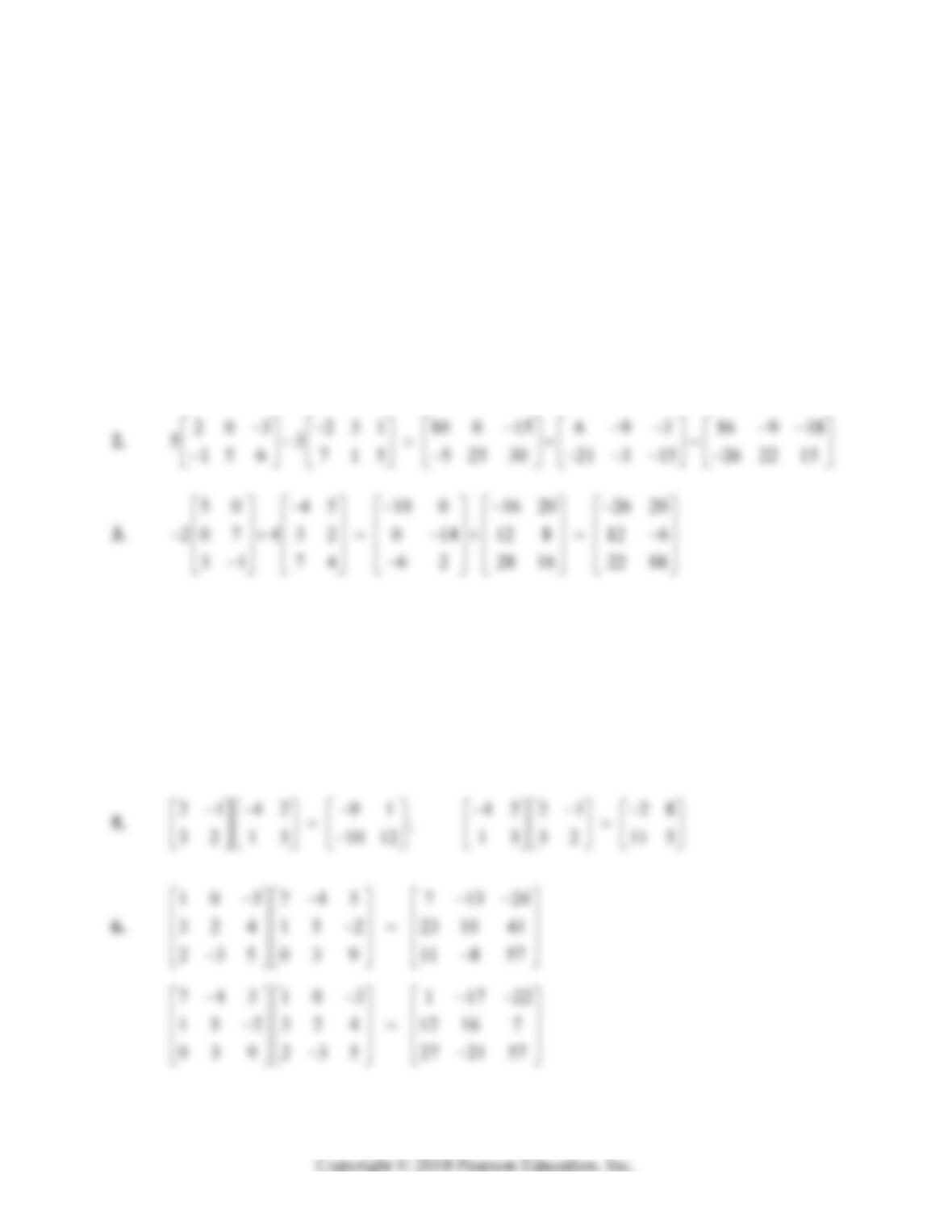
39. It is given that the augmented coefficient matrix of the homogeneous 33 system has the
form
111
222
12 12 12
0
0.
0
abc
abc
pa qa pb qb pc qc
192 Chapter 3: Linear Systems and Matrices
SECTION 3.4
MATRIX OPERATIONS
The objective of this section is simple to state. It is not merely knowledge of, but complete mastery
of matrix addition and multiplication (particularly the latter). Matrix multiplication must be
practiced until it is carried out not only accurately but quickly and with confidence — until you can
hardly look at two matrices A and B without thinking of “pouring” the ith row of A down the jth
column of B.
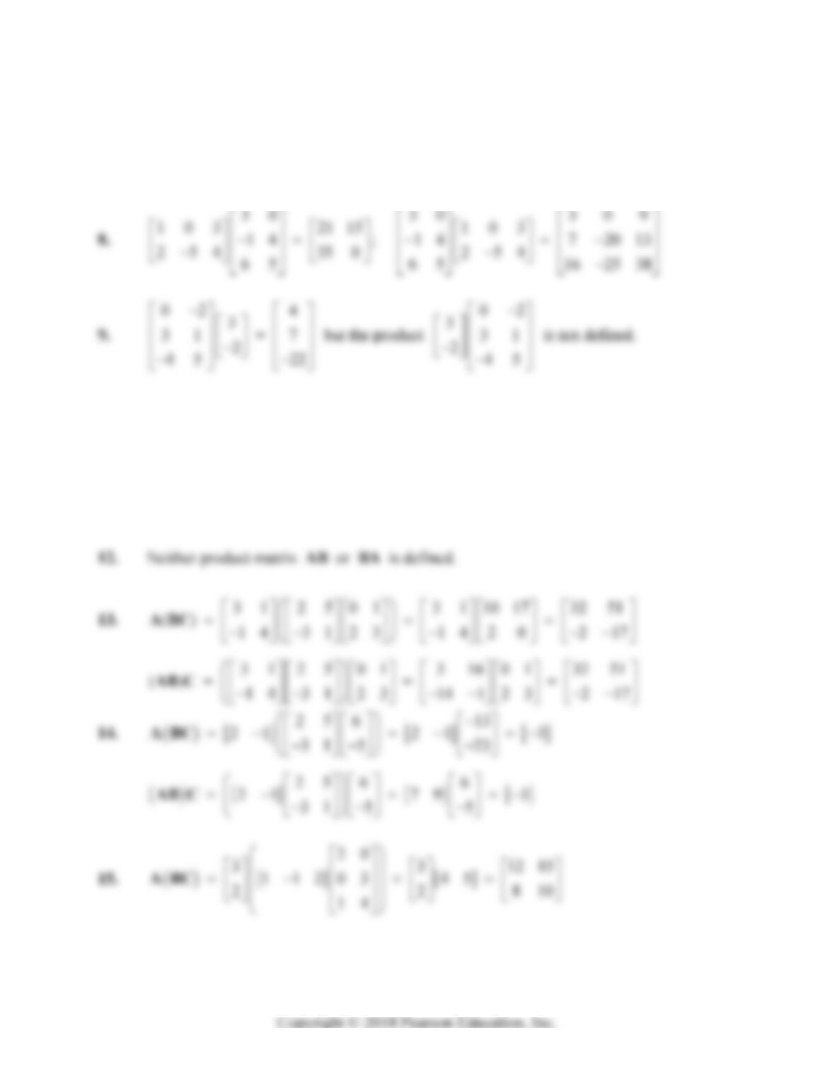
1. 35 10 915 40 5 15
34
27 3 4 621 12 16 18 5
4.
210 634
74 0 3 55 2 1
527 079
14 7 0 30 15 20 44 22 20
28 0 21 25 10 5 53 10 26
35 14 49 0 35 45 35 21 94
Section 3.4: Matrix Operations 193
7.
33369
1234 26; 4123 4 8 12
6651015
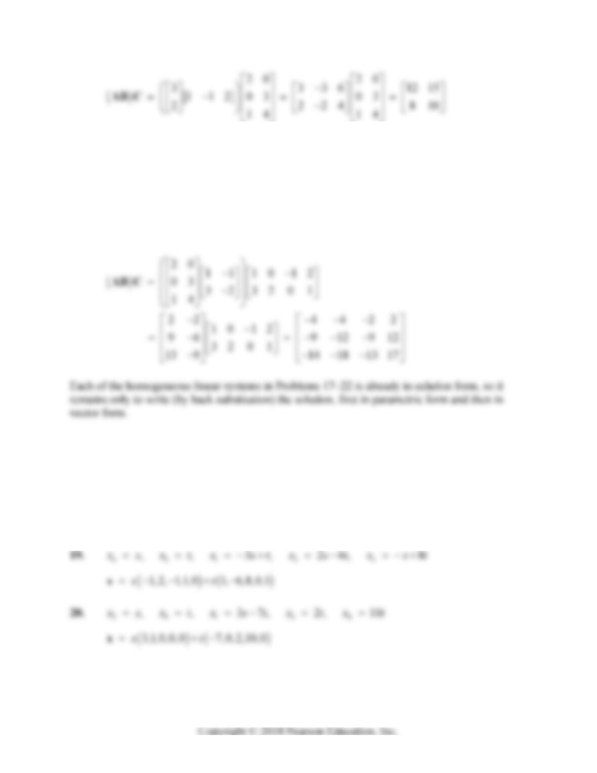
10. 21 1 0 4 1 213
43 3 25 5 631
AB but the product BA is not defined.
11.
2756
35 11153
1423
AB but the product BA is not defined.
194 Chapter 3: Linear Systems and Matrices
16.
20 111012
03 323201
14
ABC
20 4 4 2 2
2211
03 9 12 9 12
3434
1 4 14 18 13 17
17. 341 2
,,54, 27
x
sx tx stx st
5, 2,1,0 4,7,0,1st x
18. 241 3
,,36, 9
x
sx tx stx t
3,1, 0, 0 6, 0, 9,1stx
x
x