Section 3.4: Matrix Operations 195
21. 3451 2
,,, 27, 234
x
rx sx tx rstx rst
1, 2,1, 0, 0 2, 3, 0,1, 0 7, 4, 0, 0,1rst x
x
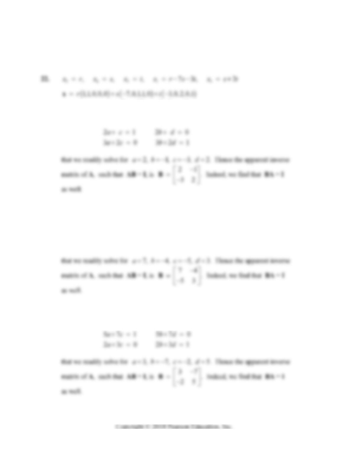
23. The matrix equation 21 10
32 01
ab
cd
entails the four scalar equations
24. The matrix equation 34 10
57 01
ab
cd
entails the four scalar equations
34 1 34 0
57 0 57 1
ac bd
ac bd
25. The matrix equation 57 10
23 01
ab
cd
entails the four scalar equations
196 Chapter 3: Linear Systems and Matrices
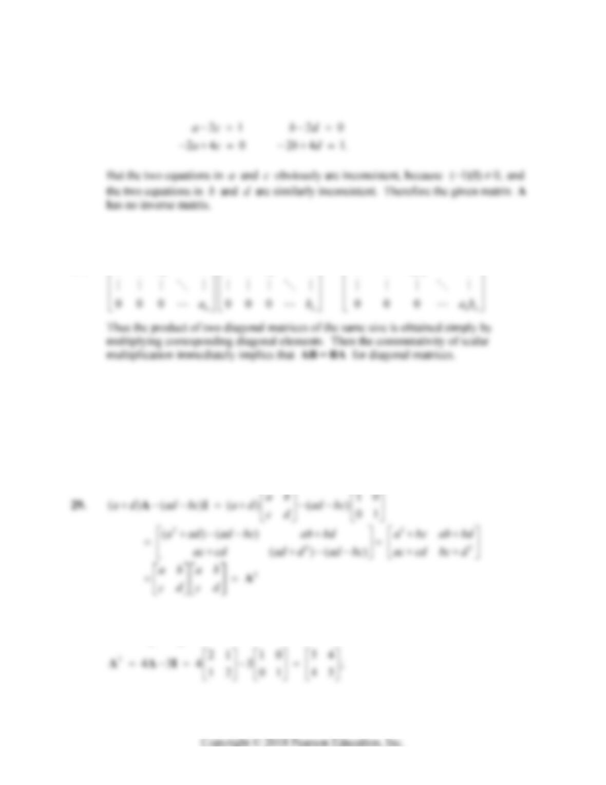
26. The matrix equation 12 10
24 01
ab
cd
entails the four scalar equations
27.
11 11
22 22
33 33
00 0 00 0 0 0 0
000000 0 0 0
00 0 00 0 0 0 0
ab ab
ab ab
ab ab
28. The matrix power n
A is simply the product AAA A of n copies of A. It follows
(by associativity) that parentheses don’t matter:
copies copies copies
()()()
rs rs
rs rs
A A AAA A AAA A AAA A A ,
the product of r + s copies of A in either case.
30. If 21
12
A then 4 and 3.a d ad bc Hence
Section 3.4: Matrix Operations 197
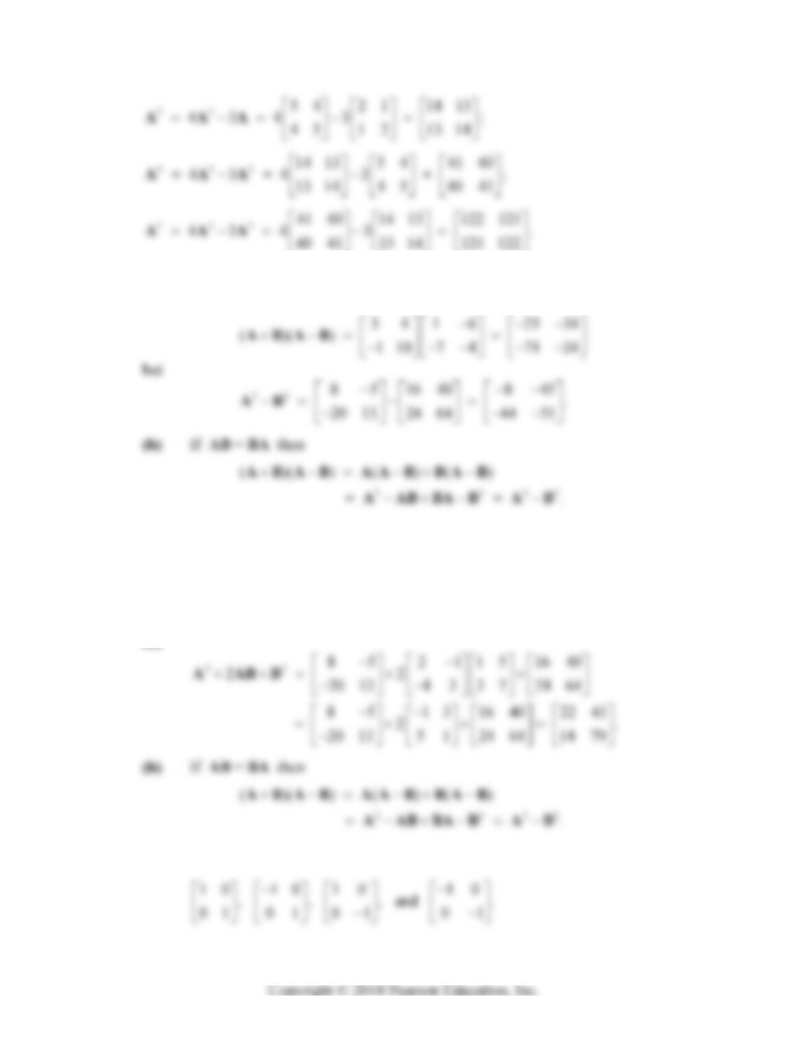
31. (a) If 21 15
and
43 37
AB then
32. (a) If 21 15
and
43 37
AB then
23434 552
() 1 10 1 10 13 96
AB
but
33. Four different 2 2 matrices A with A2 = I are
198 Chapter 3: Linear Systems and Matrices
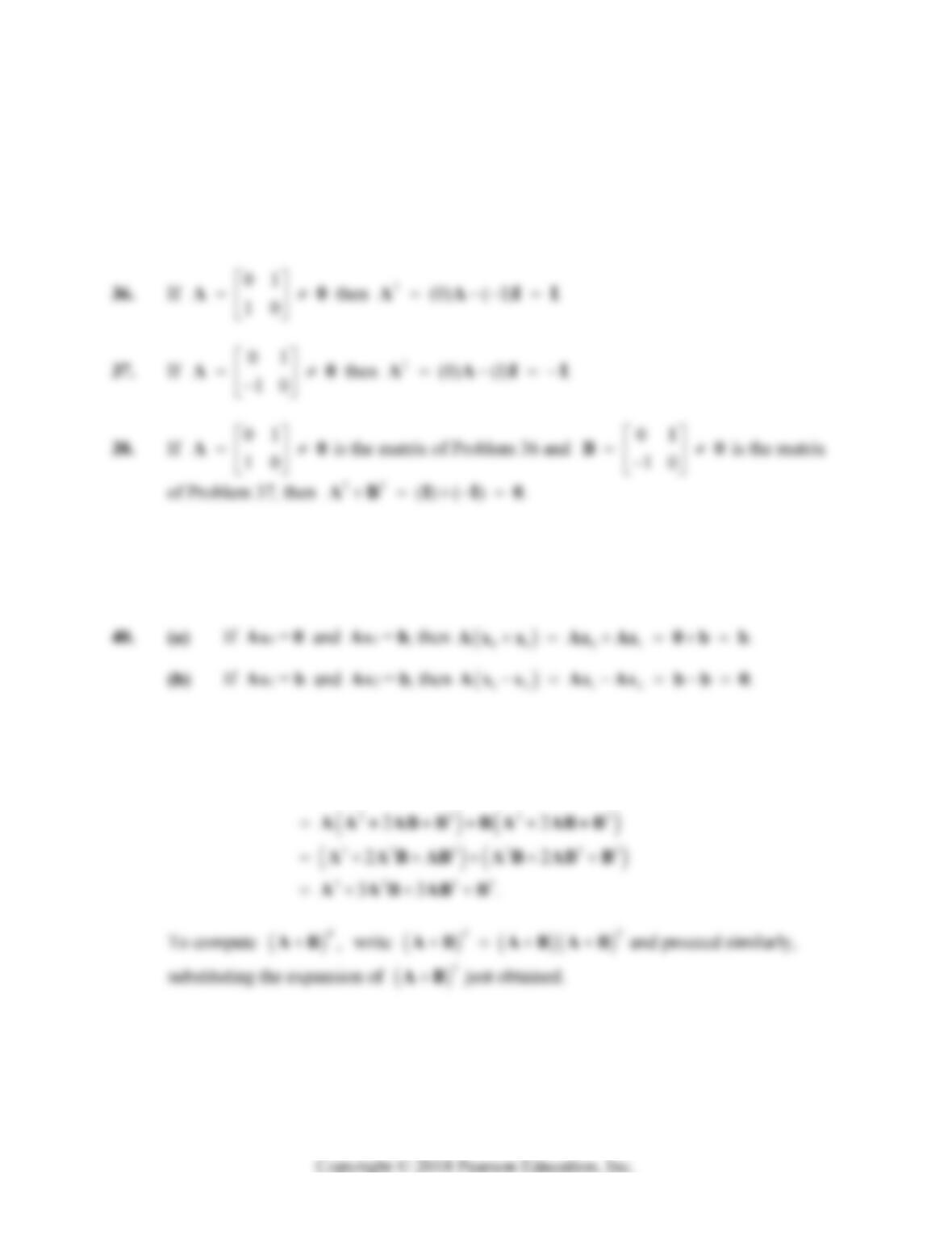
34. If 2
11 then (0) (0) .
11
A0AAI0
35. If 2
21 then (1) (0) .
21
A0AAIA
39. If Ax1 = Ax2 = 0, then
11 2 2 1 1 2 2 1 2 .cc c c c c Ax x Ax Ax 0 0 0
41. If AB = BA then
32
22
2 AB ABAB ABA ABB
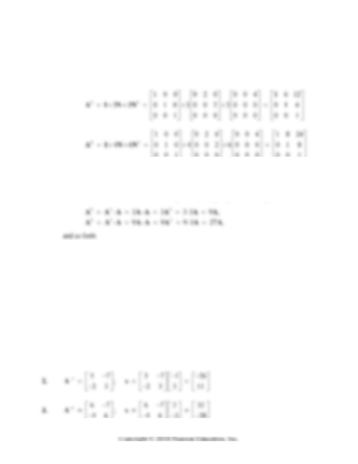
42. (a) Matrix multiplication gives 23
004 000
000 and 000.
000 000
NN
Section 3.5: Inverses of Matrices 199
(b)
22
100 020 004 144
20102002000014
001 000 000 001
AINN
001 000 000 00 1
43. First, matrix multiplication gives 2
211 633
12 1 36 3 3.
112 336
AA
Then
SECTION 3.5
INVERSES OF MATRICES
The computational objective of this section is clearcut — to find the inverse of a given invertible
matrix. From a more general viewpoint, Theorem 7 on the properties of nonsingular matrices
summarizes most of the basic theory of this chapter.
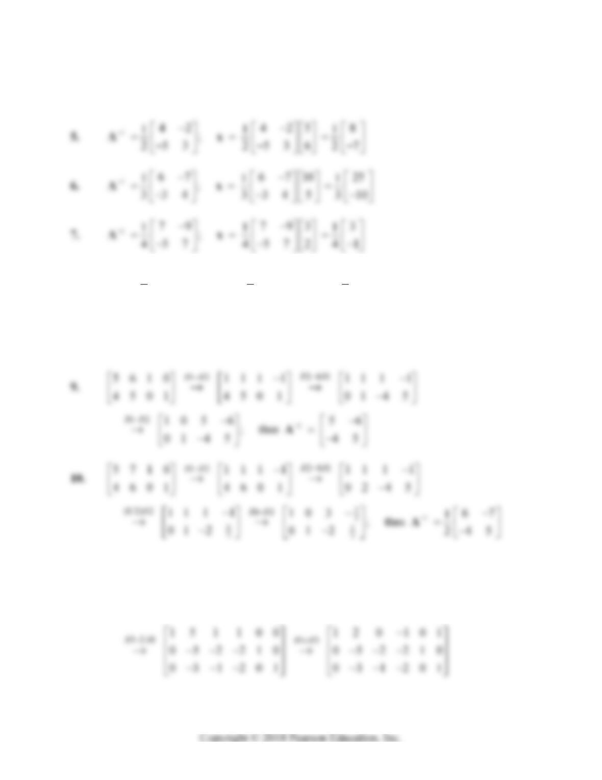
In Problems 1–8 we first give the inverse matrix 1
A and then calculate the solution vector x.
1. 132 325 3
;
43 436 2
Ax
200 Chapter 3: Linear Systems and Matrices
4. 117 12 17 12 5 25
;
75 755 10
Ax
8. 110 15 10 15 7 25
111
;
58 58 3 11
555
Ax
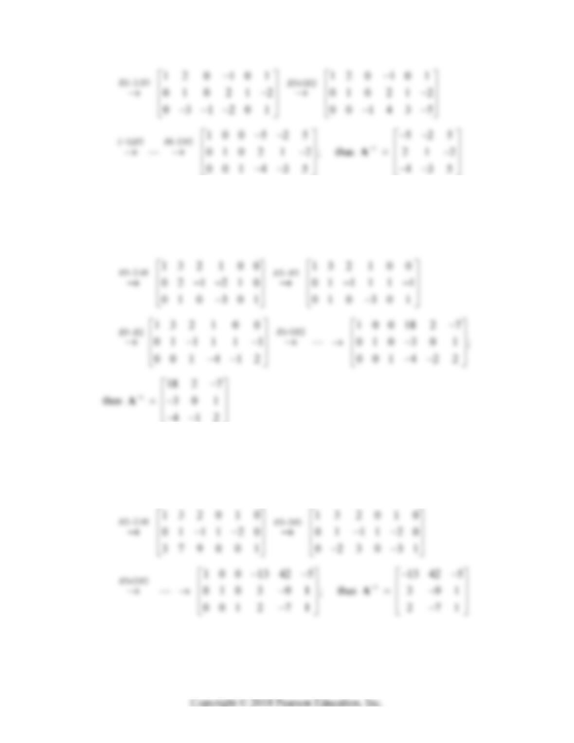
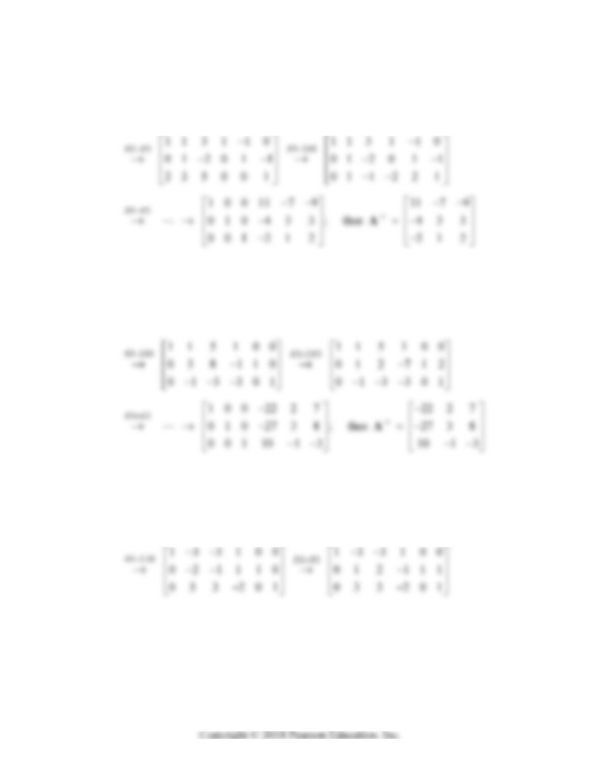
In Problems 9–22 we give at least the first few steps in the reduction of the augmented matrix
whose right half is the identity matrix of appropriate size. We wind up with its echelon form, whose
left half is an identity matrix and whose right half is the desired inverse matrix.
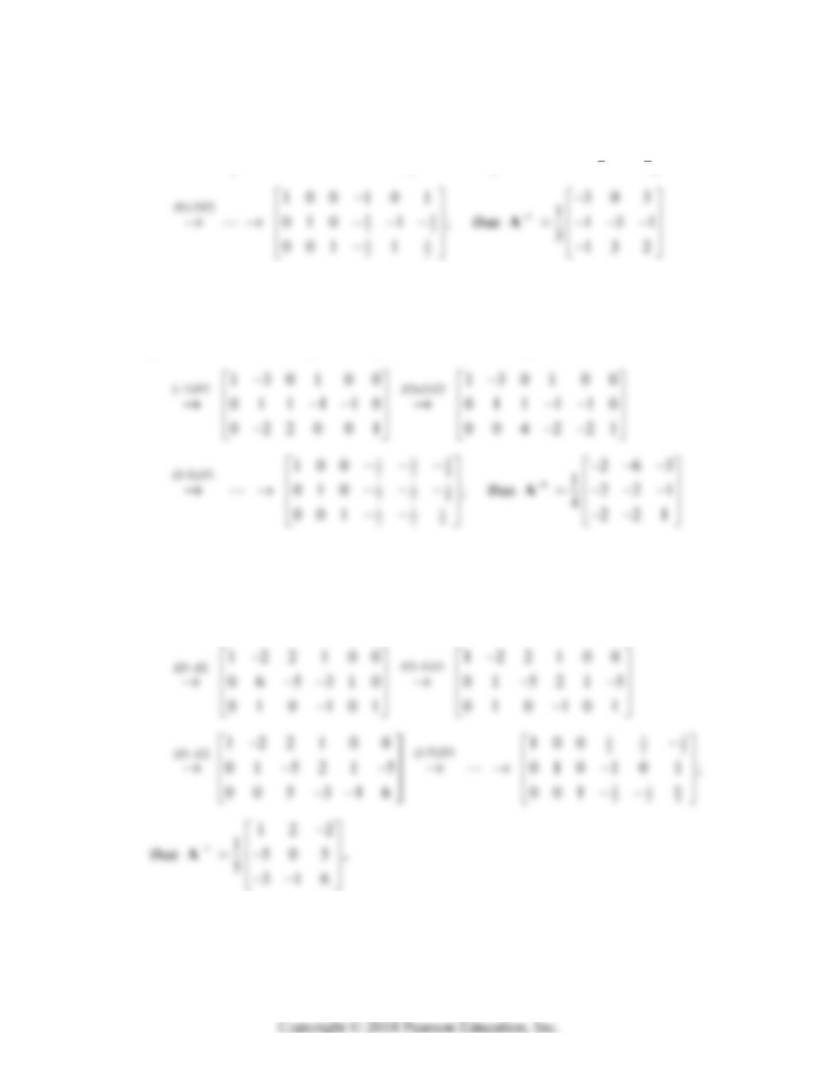
11.
221
151100 1 5 1 1 00
250010 0 5 2 210
271001 2 7 1 0 01
RR
Section 3.5: Inverses of Matrices 201
12.
221
132100 13 2 100
2 8 3010 0 2 1 210
3106001 310 6 0 01
RR
13.
(1,2)
273100 132010
132010 273100
379001 379001
SWAP R R
202 Chapter 3: Linear Systems and Matrices
14.
12
356100 1131 10
243010 2430 1 0
235001 2350 0 1
RR
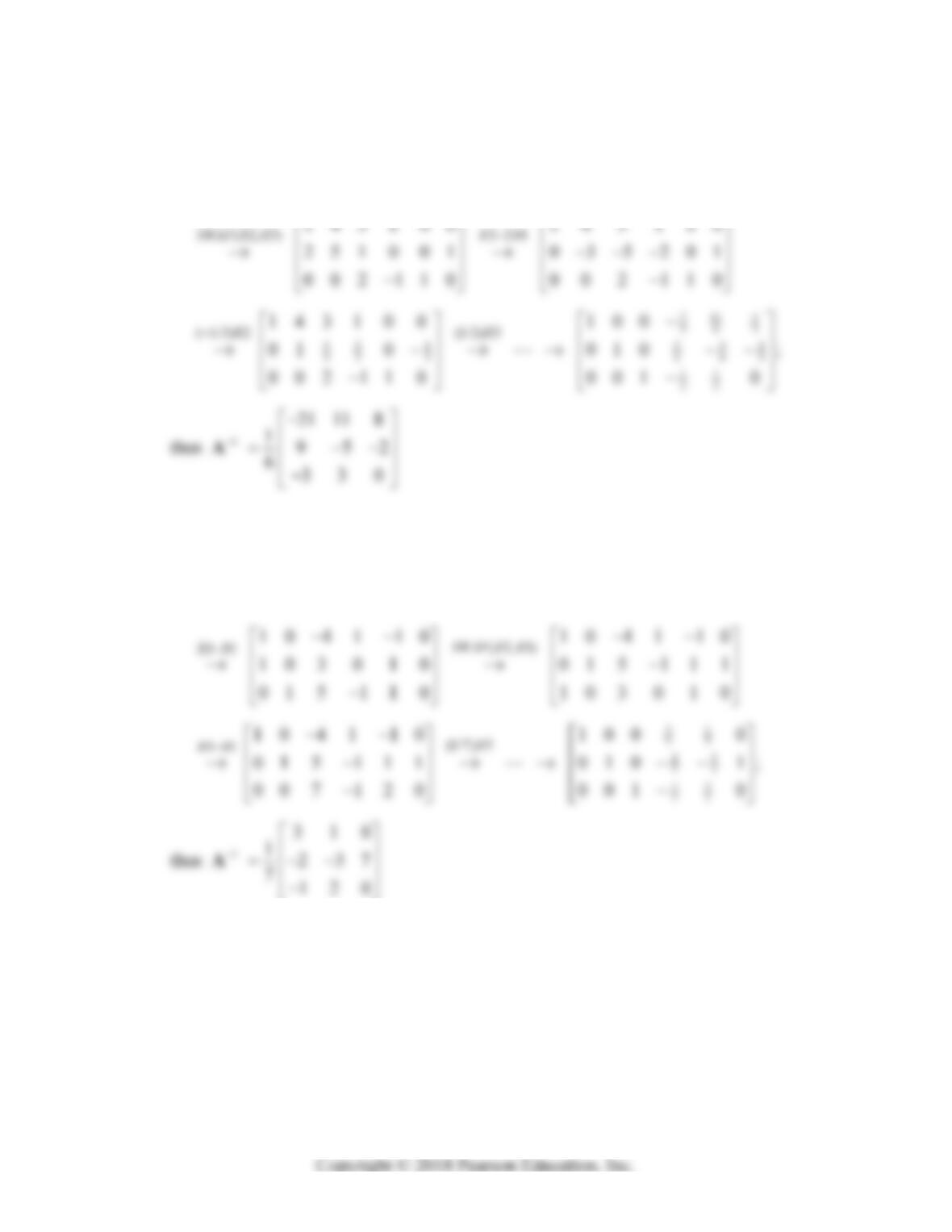
15.
21
11 5 100 11 5 1 00
1413010 03 8 110
3212001 3212001
RR
16.
21
1 3 3100 1 3 3100
1 1 2 010 0 2 1110
2 3 3001 2 3 3001
RR
Section 3.5: Inverses of Matrices 203
12
33
(1/3( 3)
33 2 133100 133100
01 2 11 1 01 2 111
00 31 3 2 00 1 1
R
RR
17.
21
1 30100 1 30100
1 2 1010 0 1 1110
0 22001 0 22001
RR
18.
231
122100 122100
3 0 1010 0 6 5 310
1 12001 1 1 2 0 01
RR
204 Chapter 3: Linear Systems and Matrices
19.
21
143100 143 1 00
145010 002 110
251001 251 0 01
RR
20.
12
20 1100 10 41 10
10 3 010 10 3 0 1 0
111001 111001
RR
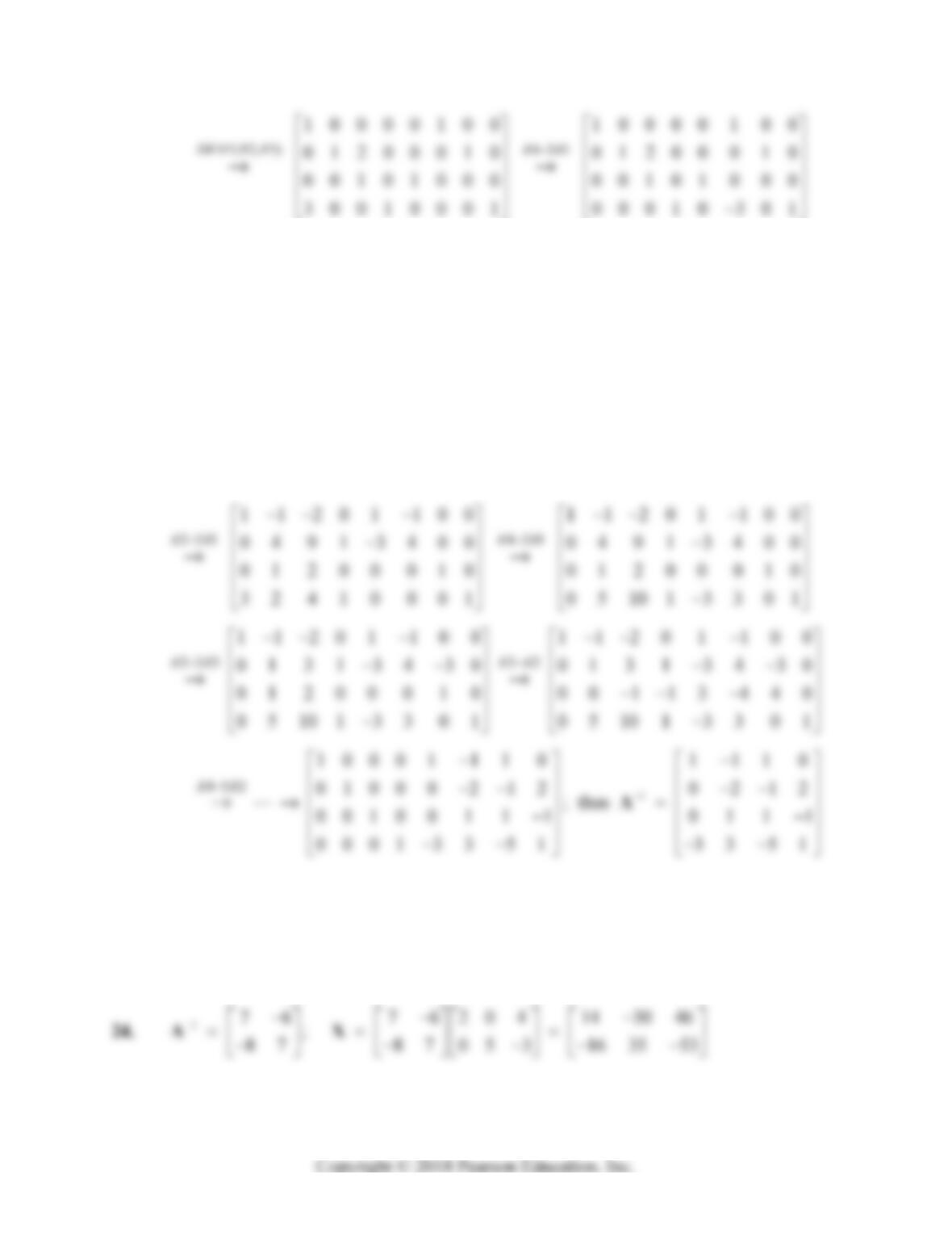
21.
(1,2)
00101000 10000100
10000100 00101000
01200010 01200010
30010001 30010001
SWAP R R
Section 3.5: Inverses of Matrices 205
223
1000 0 1 00
0100 2 0 10
;
0010 1 0 00
0001 0 301
RR
1
0100
2010
thus 1000
0301
A
22.
12
40111000 1 1 201 100
31310100 3 1 3 10 1 00
01200010 0 1 2 00 0 10
32410001 3 2 4 10 0 01
RR
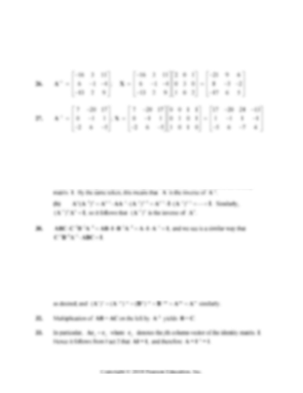
In Problems 23–28 we first give the inverse matrix 1
A and then calculate the solution matrix X.
23. 143 43135 71835
;
54 54 1 25 9 2345
AX
206 Chapter 3: Linear Systems and Matrices
25. 1
11 9 4 11 9 4 1 0 3 7 14 15
22 1; 22 1022 1 3 2
21 0 21 0 110 2 2 4
AX
28. 1
5 5 10 5 5 10 2 1 0 2 5 5 10 1
8815; 8815 1350 88157
24 23 45 24 23 45 1 1 0 5 24 23 45 13
AX
29. (a) The fact that A–1 is the inverse of A means that 11.
AA A A I That is, that
when A–1 is multiplied either on the right or on the left by A, the result is the identity
31. Let 1
0, 0, and .pr qs
BA Then
11
1
()()
(because , 0)
()
rs p q p q
pq pq
pq pq rs
pq
AA A A A A
BB B
AAA
Section 3.5: Inverses of Matrices 207
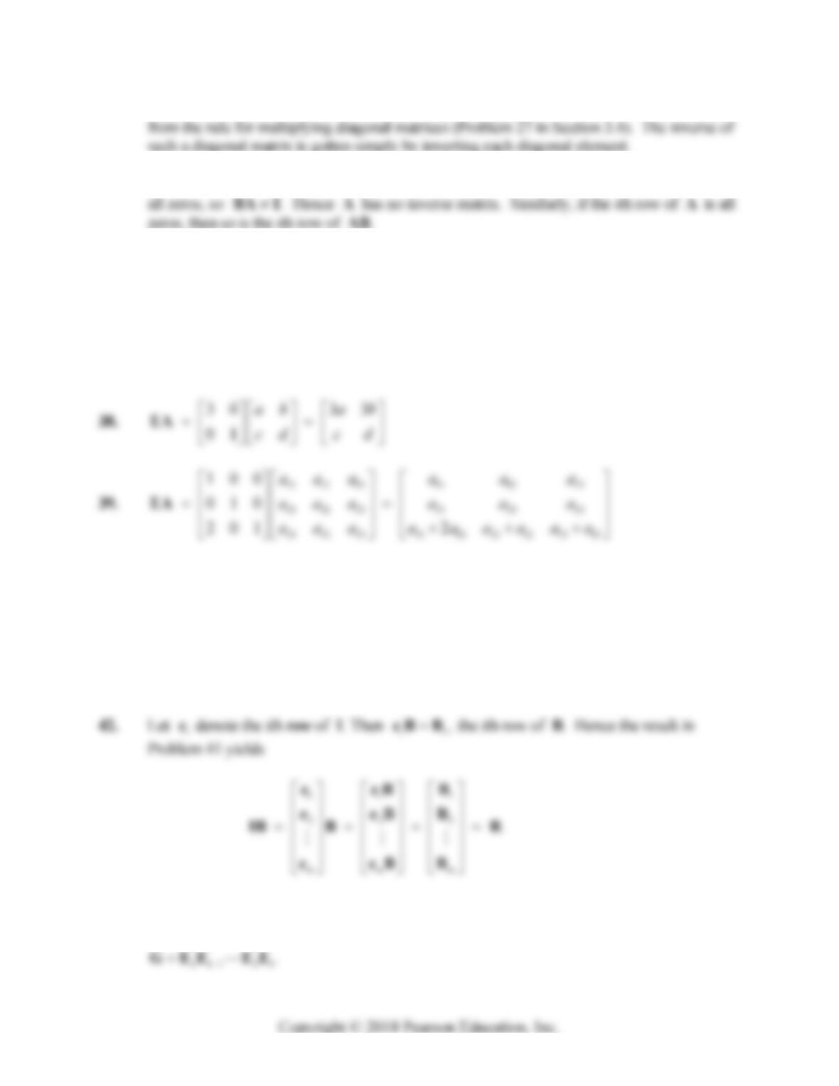
34. The invertibility of a diagonal matrix with nonzero diagonal elements follows immediately
35. If the jth column of A is all zeros and B is any nn matrix, then the jth column of BA is
36. If ad – bc = 0, then it follows easily that one row of A is a multiple of the other. Hence the
reduced echelon form of A is of the form **
00
rather than the 2 2 identity matrix.
Therefore A is not invertible.
37. Direct multiplication shows that 11.
AA A A I
40.
11 12 13 21 22 23
21 22 23 11 12 13
31 32 33 31 32 33
010
100
001
aaa aaa
aaa aaa
aaa aaa
EA
41. This follows immediately from the fact that the ijth element of AB is the product of the ith
row of A and the jth column of B.
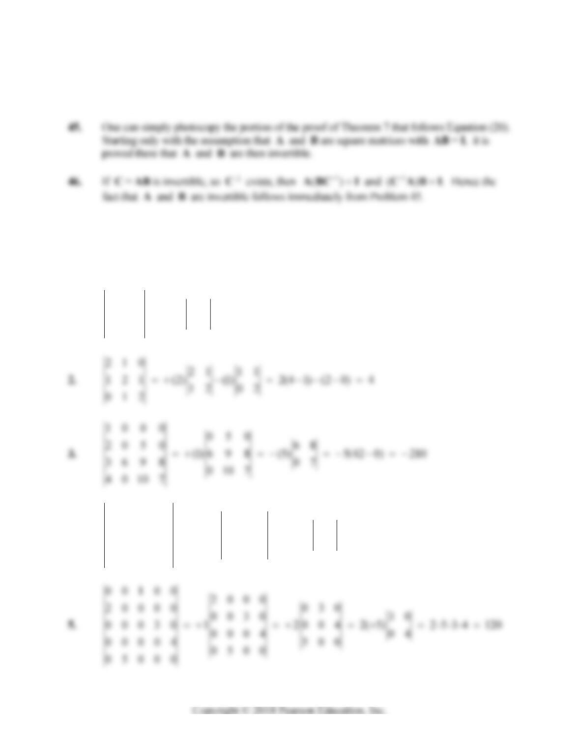
43. Let 12
,, ,
k
EE E be the elementary matrices corresponding to the elementary row
operations that reduce A to B. Then Theorem 5 gives 121kk
BEE EEAGA where
208 Chapter 3: Linear Systems and Matrices
44. This follows immediately from the result in Problem 43, because an invertible matrix is
row-equivalent to the identity matrix.
SECTION 3.6
DETERMINANTS
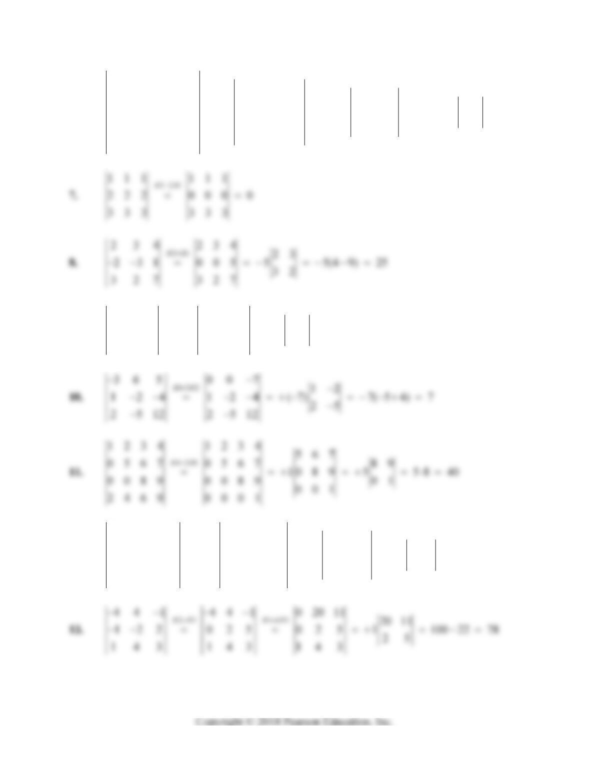
1.
003 40
400 (3) 345 60
05
050
4.
5118 7 5118
32623 58
( 3) 3 2 6 3( 4) 12(30 24) 72
000 3 36
040
04017
Section 3.6: Determinants 209
6.
3011 50 30 50 300
2413 6 5 24 6 5 45
5 5( 2) 2 4 5 10( 3) 60
005 00 76177 67
767
76 9177 0020
008 20
9.
321
325 325 35
0 5 17 0 5 17 2 5(6 0) 30
02
6412 002
RR
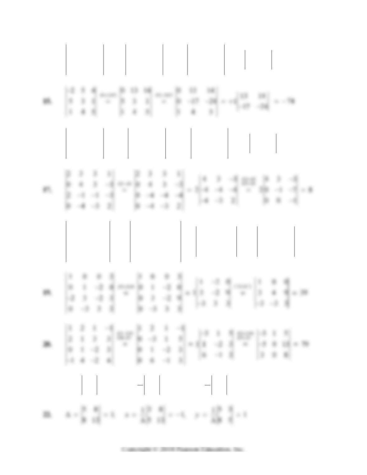
12.
421
200 3 200 3 11112
0 1 11 12 0 1 11 12 5 13
20 5 13 2 2 5 10
00513 00513 01
00 1
4007 0001
RR
210 Chapter 3: Linear Systems and Matrices
14.
231
351
12
42 2 113 11 3 214
31 5 31 5 0214 1 22
118
543 543 0118
RR
RR
RR
16.
12 3 22 3
24 2 100 4 1004 10 4
541 541 1301 2 84
13 1
42 1 42 1 421
RR R R
18.
291
331 3 1
14 4 1 1 4 4 1 122 122
01 2 2 0 1 2 2 1 9 11 1 0 29 19 135
3314 09111 132 014
01 3 2 0 1 3 2
RR
RR RR
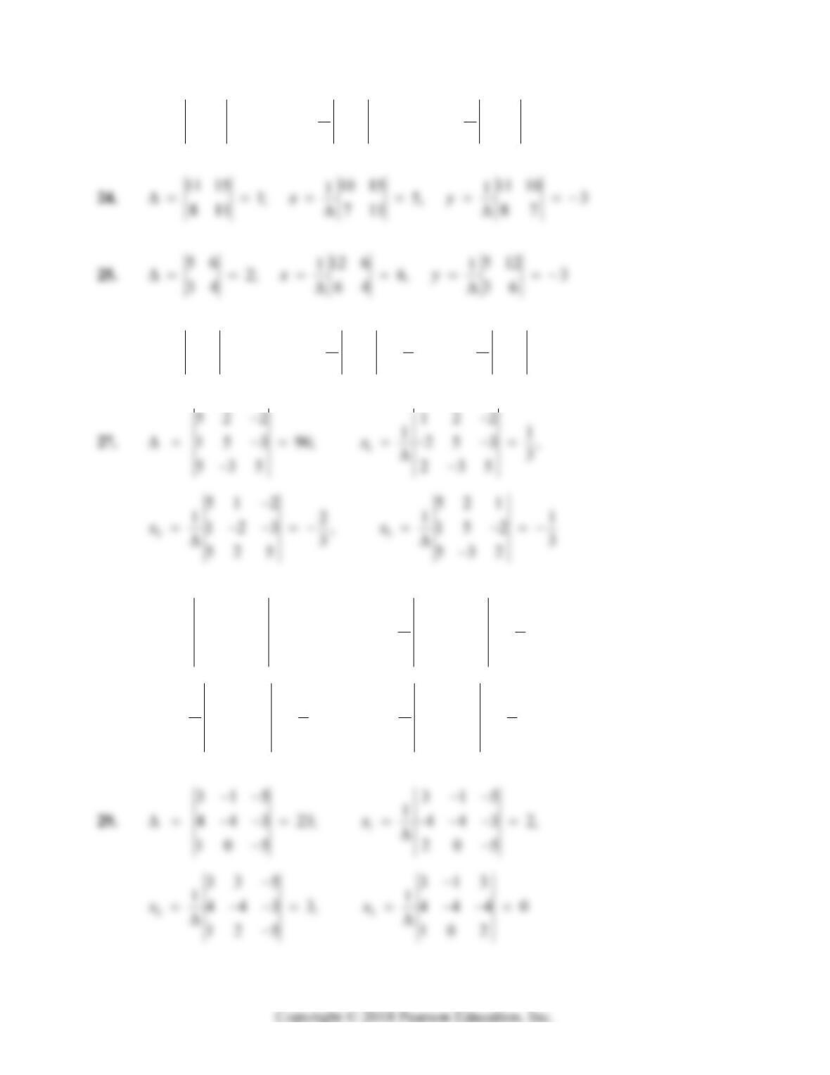
21. 34 24 32
11
1; 10, 7
57 17 51
xy
Section 3.6: Determinants 211
23. 17 7 6 7 17 6
11
1; 2, 4
12 5 4 5 12 4
xy
26. 67 37 63
111
2; , 0
89 49 84
2
xy
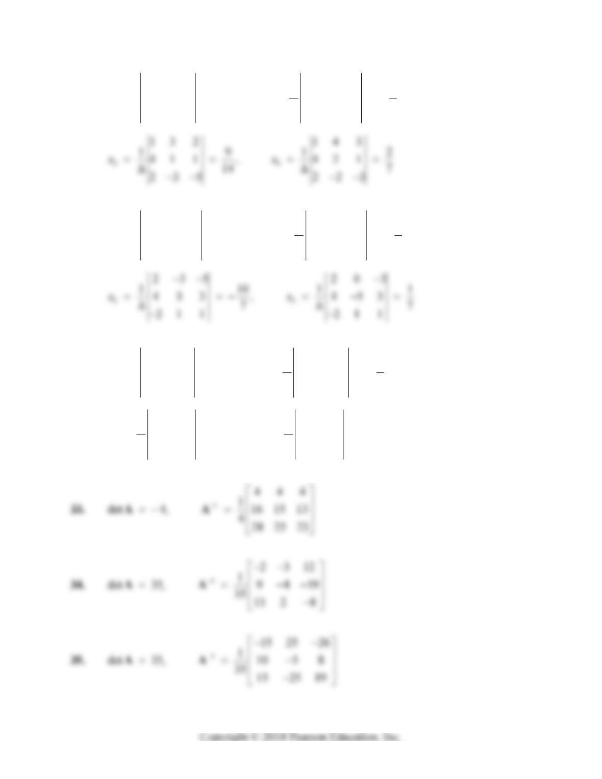
28. 1
54 2 44 2
14
20 3 35; 20 3 ,
7
211 111
x
23
54 2 5 4 4
1312
22 3 , 2 0 2
77
21 1 2 11
xx
212 Chapter 3: Linear Systems and Matrices
30. 1
14 2 3 4 2
11
42 1 56; 1 2 1 ,
7
225 325
x
31. 1
20 5 30 5
18
453 14; 353 ,
7
21 1 1 1 1
x
32. 1
34 3 54 3
17
324 6; 724 ,
3
32 1 32 1
x
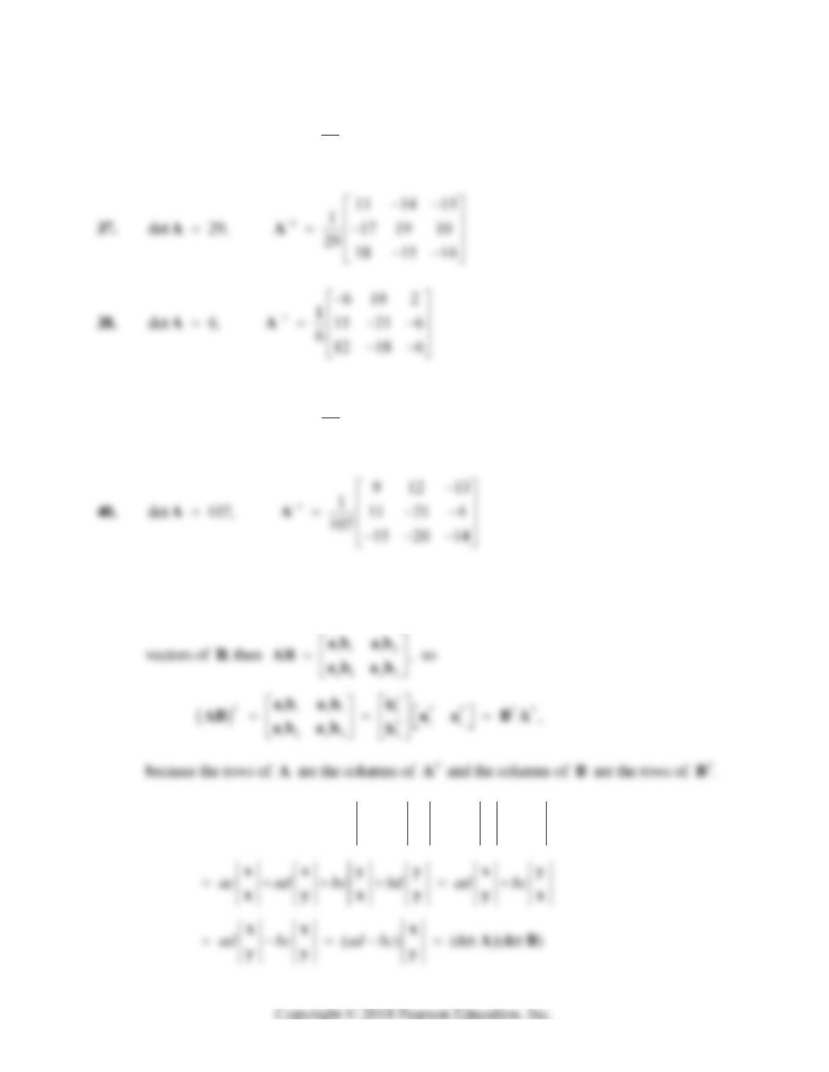
23
35 3 3 4 5
11
37 4 9, 3 27 8
33 1 3 2 3
xx
Section 3.6: Determinants 213
36. 1
520 17
1
det 23, 10 17 11
23 14 8
AA
39. 1
21 1 13
1
det 37, 4 9 6
37 65 9
AA
41. If
1
12
2
and
a
ABbb
a in terms of the two row vectors of A and the two column
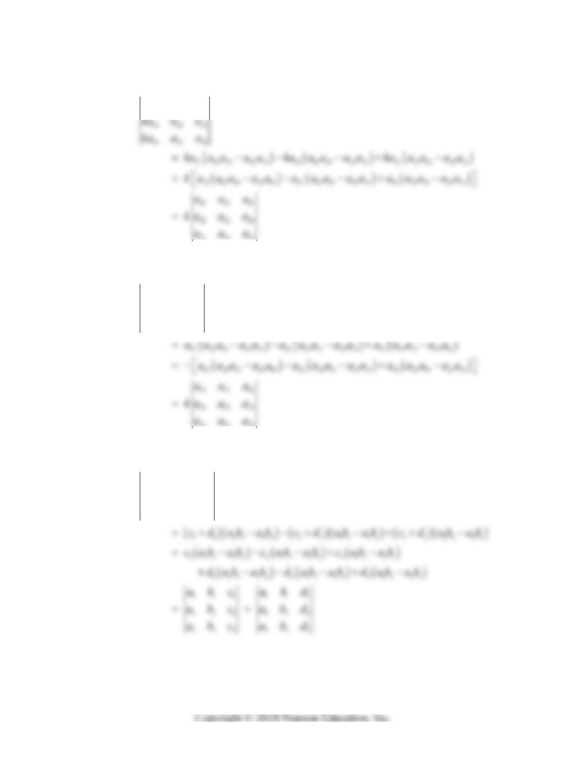
42. det det ab a b a b
cd cd cd cd
xx
y
x
y
AB
y
x
y
x
y
x
y
214 Chapter 3: Linear Systems and Matrices
43. We expand the left-hand determinant along its first column:
11 12 13
ka a a
44. We expand the left-hand determinant along its third row:
21 22 23
11 12 13
31 32 33
aaa
aaa
aaa
45. We expand the left-hand determinant along its third column:
1111
222 2
3333
abcd
abcd
abcd