Section 1.2: Integrals as General and Particular Solutions 15
42. Let ()
x
t be the (positive) altitude (in miles) of the spacecraft at time t (hours), with 0t
corresponding to the time at which its retrorockets are fired; let
vt x t
be the veloc-
ity of the spacecraft at time t. Then 01000v and
00xx is unknown. But the
x
43. The velocity and position functions for the spacecraft are
0.0098
S
vt t and
2
0.0049
S
x
tt, and the corresponding functions for the projectile are
x
44. Let 0a denote the constant deceleration of the car when braking, and take 00x for
the car’s position at time 0t when the brakes are applied. In the police experiment
with 025v ft/s, the distance the car travels in t seconds is given by
2
188
25
260
x
tat t ,
x
45. Equation (10) gives
22
22222
000 00
2vt v at v v at atv v 2
0
v22
0
2at atv ,
whereas by Eq. (11),
16 Chapter 1: First-Order Differential Equations
SECTION 1.3
SLOPE FIELDS AND SOLUTION CURVES
The instructor may choose to delay covering Section 1.3 until later in Chapter 1. However, be-
fore proceeding to Chapter 2, it is important that students come to grips at some point with the
question of the existence of a unique solution of a differential equation –– and realize that it
makes no sense to look for the solution without knowing in advance that it exists. It may help
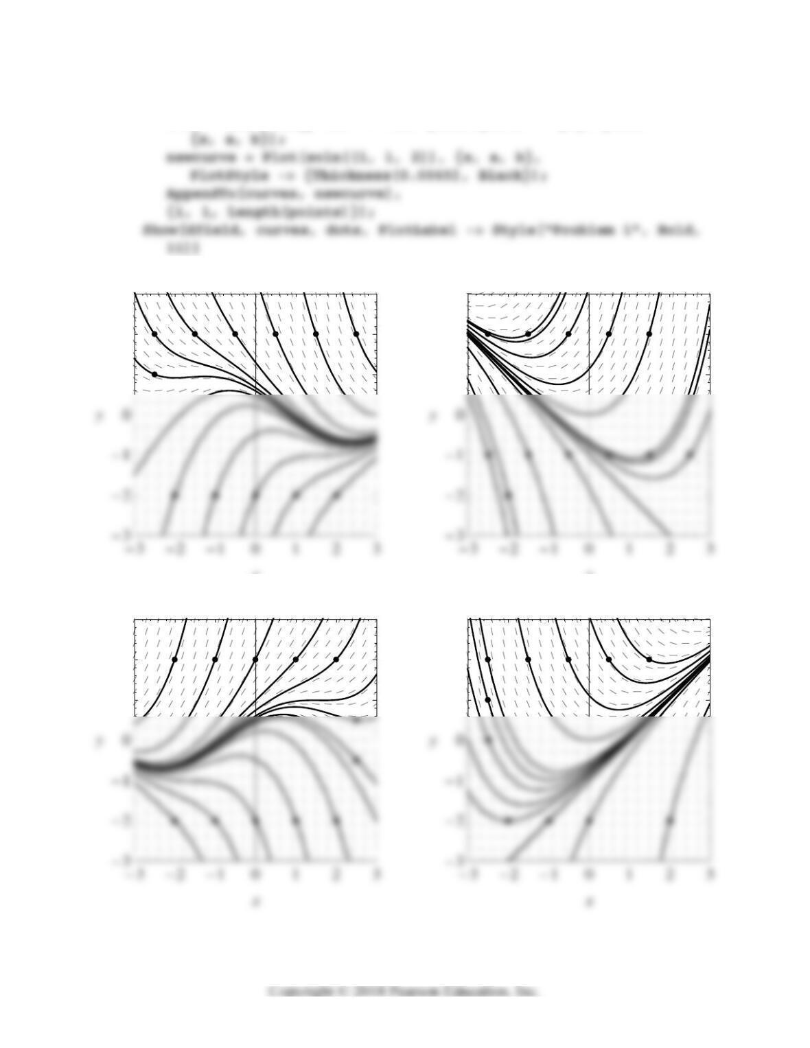
1. The following sequence of Mathematica 7 commands generates the slope field and the
solution curves through the given points. Begin with the differential equation
/,dy dx f x y, where
Section 1.3: Slope Fields and Solution Curves 17
The original curve shown in Fig. 1.3.15 of the text (and its initial point not shown there)
are plotted by the commands
x0 = -1.9; y0 = 0;
point0 = Graphics[{PointSize[0.025], Point[{x0, y0}]}];
soln = NDSolve[{y'[x] == f[x, y[x]], y[x0] == y0}, y[x],
{x, a, b}];
curve0 = Plot[soln[[1, 1, 2]], {x, a, b}, PlotStyle ->
x0 = -2.5; y0 = 1;
point7 = Graphics[{PointSize[0.025], Point[{x0, y0}]}];
soln = NDSolve[{y'[x] == f[x, y[x]], y[x0] == y0}, y[x],
{x, a, b}];
curve7 = Plot[soln[[1, 1, 2]], {x, a, b},
PlotStyle -> {Thickness[0.0065], Blue}];
Show[curve7, point7]
The following command superimposes the two solution curves and starting points found
so far upon the slope field:
18 Chapter 1: First-Order Differential Equations
dots = AppendTo[dots, newdot];
soln = NDSolve[{y'[x] == f[x, y[x]],y[x0] == y0}, y[x],
1
2
3
x
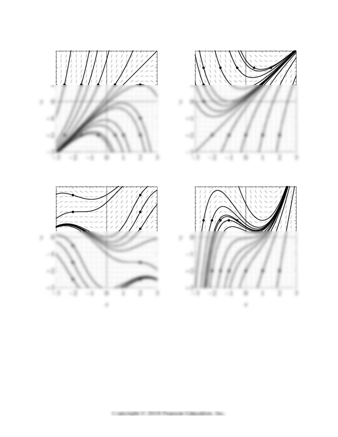
Problem 1
1
2
3
x
Problem 2
1
2
3
Problem 3
1
2
3
Problem 4
Section 1.3: Slope Fields and Solution Curves 19
2
3
x
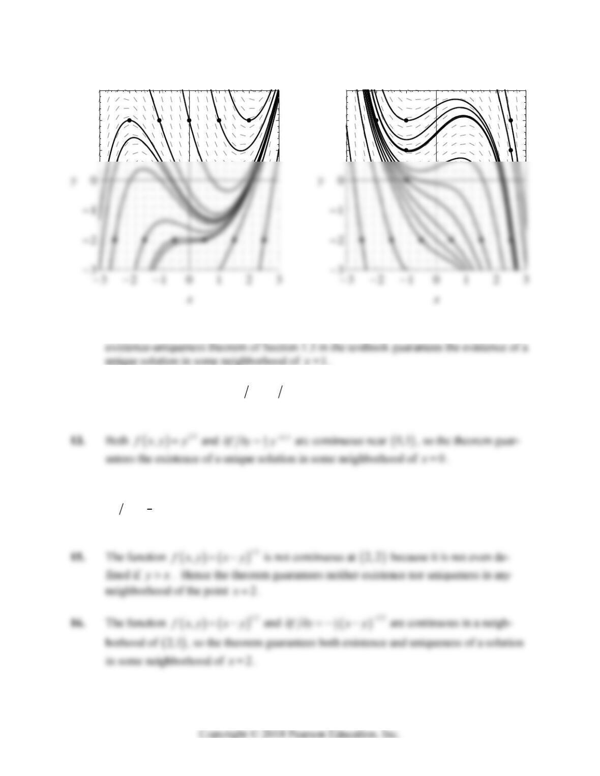
Problem 5
2
3
x
Problem 6
1
2
3
Problem 7
1
2
3
Problem 8
20 Chapter 1: First-Order Differential Equations
11. Because both
22
,2
f
xy xy and
2
,4
y
D
fxy xy are continuous everywhere, the
x
12. Both
,ln
f
x
yxy and
f
yxy are continuous in a neighborhood of
1, 1 , so the
theorem guarantees the existence of a unique solution in some neighborhood of 1
x
.
f
f
14. The function
1/3
,
f
xy y is continuous in a neighborhood of
0, 0 , but
2/3
1
3
f
yy
is not, so the theorem guarantees existence but not uniqueness in some
neighborhood of 0x. (See Remark 2 following the theorem.)
1
2
3
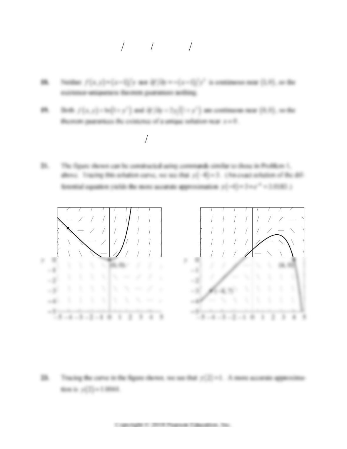
Problem 9
1
2
3
Problem 10
Section 1.3: Slope Fields and Solution Curves 21
17. Both
,1
f
xy x y and
2
1
f
yxy are continuous near
0,1 , so the
theorem guarantees both existence and uniqueness of a solution in some neighborhood of
0x.
f
f
20. Both
22
,
f
xy x y and 2
f
yy are continuous near
0,1 , so the theorem
guarantees both existence and uniqueness of a solution in some neighborhood of 0x.
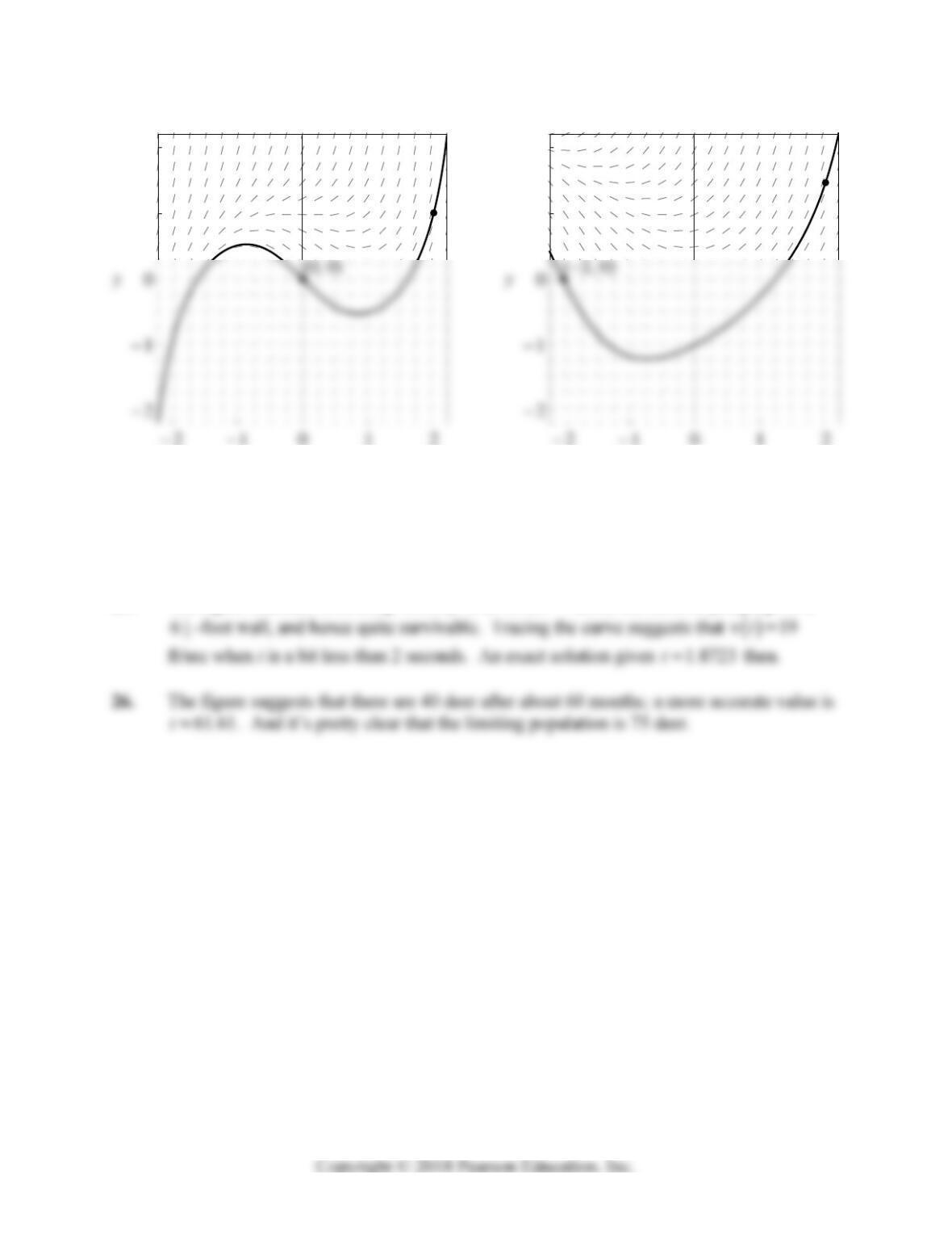
22. Tracing the curve in the figure shown, we see that
43y
. An exact solution of the
differential equation yields the more accurate approximation
43.0017y .
4, ?
1
2
3
4
5
x
Problem 21
1
2
3
4
5
x
Problem 22
22 Chapter 1: First-Order Differential Equations
24. Tracing the curve in the figure shown, we see that
21.5y. A more accurate approx-
imation is
21.4633y.
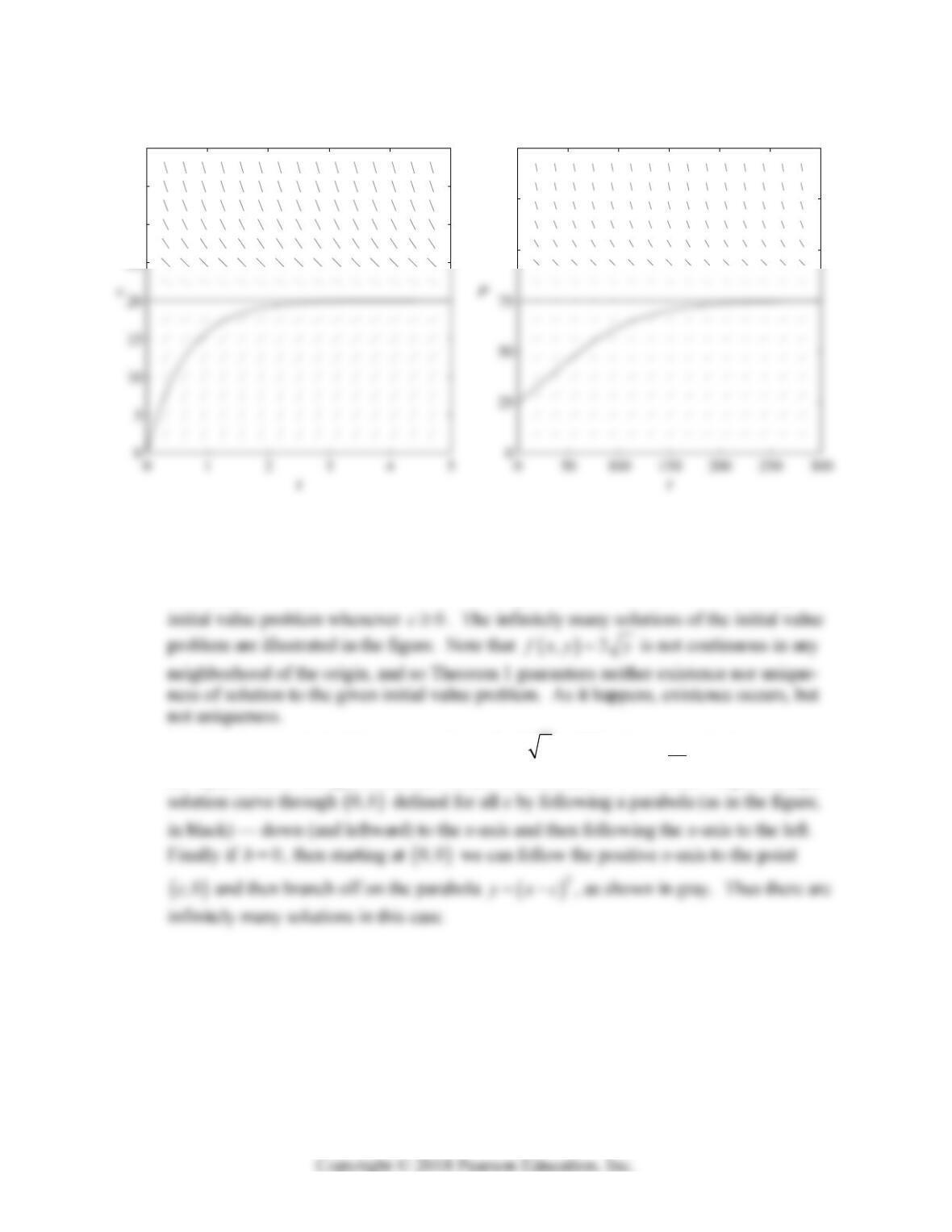
25. The figure indicates a limiting velocity of 20 ft/sec — about the same as jumping off a
2, ?
1
2
x
Problem 23
2, ?
1
2
x
Problem 24
Section 1.3: Slope Fields and Solution Curves 23
27. a) It is clear that
yx satisfies the differential equation at each x with
x
c or
x
c
,and by examining left- and right-hand derivatives we see that the same is true at
x
c.
Thus
yx not only satisfies the differential equation for all x, it also satisfies the given
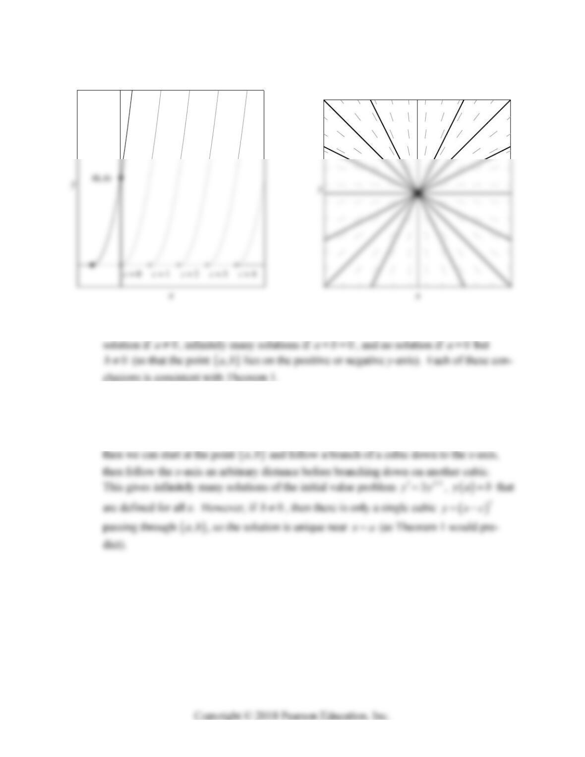
b) If 0b, then the initial value problem 2yy
,
0yb has no solution, because
the square root of a negative number would be involved. If 0b, then we get a unique
30
35
40
Problem 25
100
125
150
Problem 26
24 Chapter 1: First-Order Differential Equations
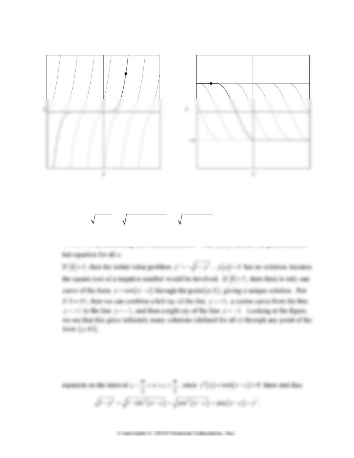
28. The figure makes it clear that the initial value problem
xy y
,
ya b has a unique
29. As with Problem 27, it is clear that
yx satisfies the differential equation at each x with
x
c or
x
c, and by examining left- and right-hand derivatives we see that the same is
true at
x
c. Looking at the figure on the left below, we see that if, for instance, 0b,
x
Problem 27a
Problem 28
Section 1.3: Slope Fields and Solution Curves 25
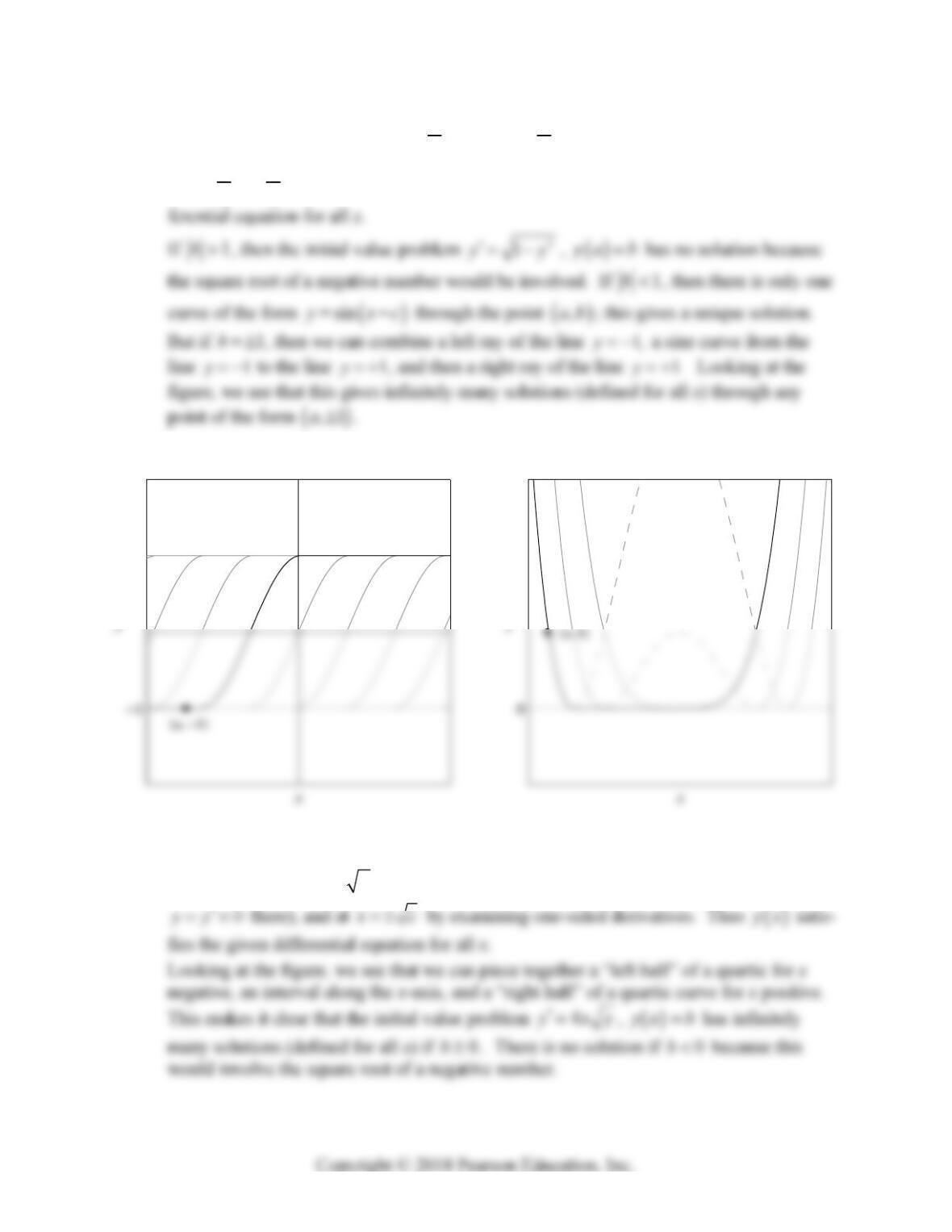
30. The function
yx satisfies the given differential equation on the interval cxc
,
since
sin 0yx xc
there and thus
22 2
11cos sin sin
y
xc xc xc y
.
Moreover, the same is true for
x
c and
x
c
(since 21y and 0y there), and at
,
x
cc
yx satisfies the given differen-
31. The function
1if /2
sin if /2 /2
1if /2
xc
yx x c c x c
xc
satisfies the given differential
(a, b)
Problem 29
1
(a, +1)
Problem 30
26 Chapter 1: First-Order Differential Equations
Moreover, the same is true for 2
x
and 2
xc
(since 21y and 0y there), and
at ,
22
xc
by examining one-sided derivatives. Thus
yx satisfies the given dif-
32. The function
yx satisfies the given differential equation for 2
x
c, since
2
44
y
xxxcx
y
there. Moreover, the same is true for 2
x
c (since
1
Problem 31
Problem 32
Section 1.3: Slope Fields and Solution Curves 27
33. Looking at the figure provided in the answers section of the textbook, it suffices to ob-
serve that, among the pictured curves
/1yxcx
for all possible values of c,
there is a unique one of these curves through any point not on either coordinate axis;
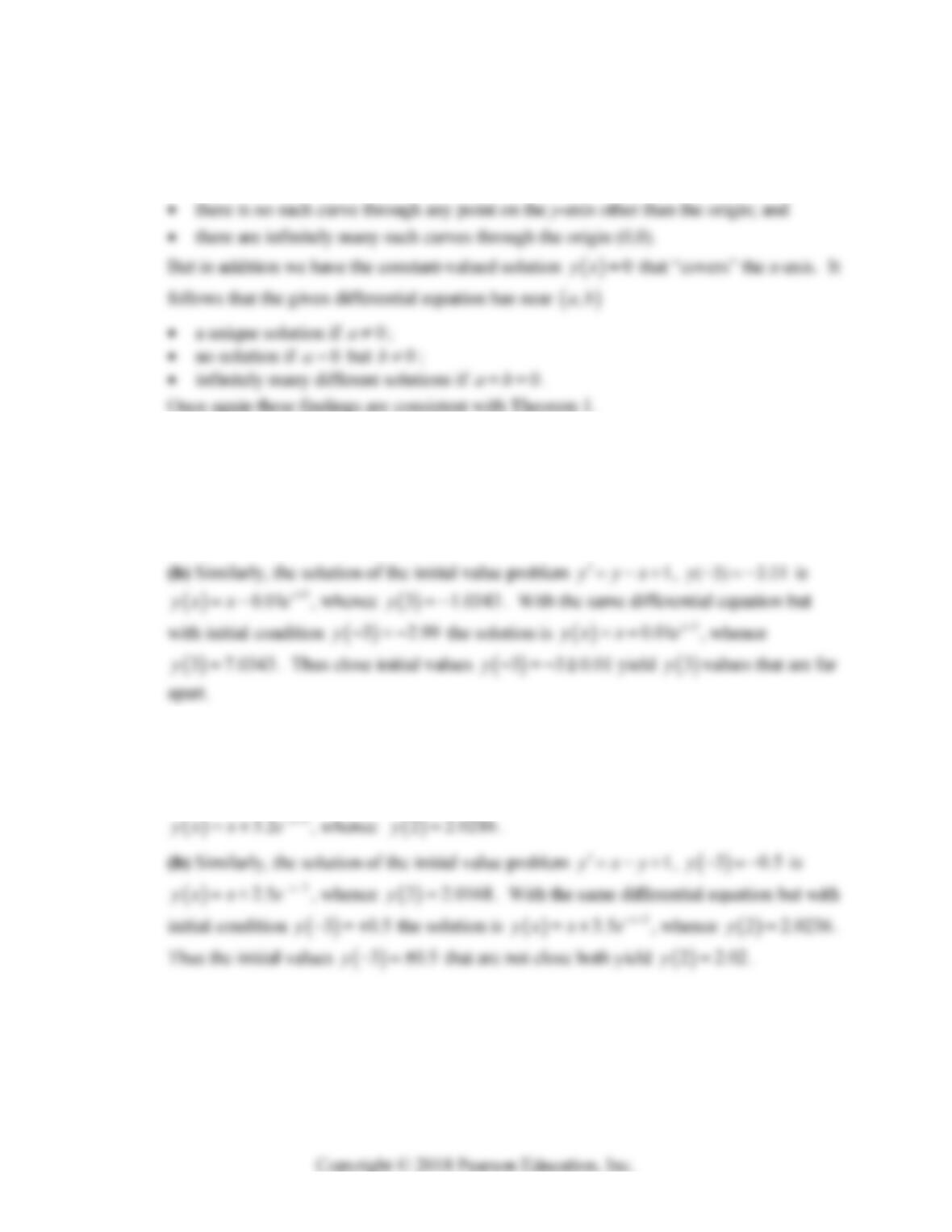
34. (a) With a computer algebra system we find that the solution of the initial value problem
1
yy
x
,
11.2y is
1
0.2
x
yx x e
, whence
10.4778y . With the
same differential equation but with initial condition
10.8y the solution is
1
0.2
x
yx x e
, whence
12.4778y
yy
x
x
35. (a) With a computer algebra system we find that the solution of the initial value problem
1
y
x
y
,
30.2y is
3
2.8
x
yx x e
, whence
2 2.0189y. With the
same differential equation but with initial condition
30.2y the solution is
x
y
y
x
x
28 Chapter 1: First-Order Differential Equations
SECTION 1.4
SEPARABLE EQUATIONS AND APPLICATIONS
Of course it should be emphasized to students that the possibility of separating the variables is
the first one you look for. The general concept of natural growth and decay is important for all
differential equations students, but the particular applications in this section are optional. Torri-
celli’s law in the form of Equation (24) in the text leads to some nice concrete examples and
problems.
Also, in the solutions below, we make free use of the fact that if C is an arbitrary constant, then
so is 53C, for example, which we can (and usually do) replace simply with C itself. In the
same way we typically replace C
e by C, with the understanding that C is then an arbitrary non-
zero constant.
1. For 0y separating variables gives 2
dy
x
dx
y
, so that 2
ln yxC , or
x
x
3. For 0y separating variables gives sin
dy
x
dx
y
, so that ln cosyxC , or
cos cos
x
Cx
yx e Ce
, where C is an arbitrary nonzero constant. (The equation also
has the singular solution 0y.)
Section 1.4: Separable Equations and Applications 29
6. For
,0xy
separating variables gives 3
dy
x
dx
y
, so that 3/2
22yx C
, or
2
3/2
y
xxC. For
,0xy
we write
3
dy
x
y
dx
, leading to
3
dy
x
dx
y
, or
3/2
22
y
xC
, or
2
3/2
yx x C
.
x
y
y
y
9. For 0y separating variables and decomposing into partial fractions give
2
211
111
dy dx dx
y
xxx
, so that ln ln 1 ln 1yxxC
, or
1
1
x
yC
x
, where C is an arbitrary positive constant, or
1
1
x
yx C
x
, where C is an
arbitrary nonzero constant. (The equation also has the singular solution 0y.)
11. For 0y separating variables gives 3
dy
x
dx
y
, so that
2
2
1
22
xC
y
, or
30 Chapter 1: First-Order Differential Equations
12. Separating variables gives 21
yd
y
xdx
y
, so that
22
11
ln 1
22
yxC , or
2
21
x
yCe , or 21
x
yCe , where C is an arbitrary nonzero constant.
15. For 0x and 2
0, 2
y separating variables gives 24 2
21 11
d
y
dx
yy xx
, so that
3
21 1
ln
3
x
C
yy x
, where C is an arbitrary constant.
y
18. Factoring gives
2222222
111
xy
x
y
x
y
x
y
, and then for 0x separating
variables gives 22
11
1
1d
y
dx
yx
, so that 11
tan yxC
x
, or
1
tanyx C x
x
, where C is an arbitrary nonzero constant.
y
Section 1.4: Separable Equations and Applications 31
20. Separating variables gives 2
2
13
1d
y
xdx
y
, or 13
tan
y
xC
. The initial condi-
tion
01y implies that 4
C
, leading to the particular solution
3
tan 4
yx x
.
22. For 0y separating variables gives 3
141d
y
xdx
y
, so that 4
ln yxxC
, or
x
23. Rewriting the differential equation as 21
dy y
dx
, we see that for 1
2
y separating vari-
ables gives 1
21
d
y
dx
y
, so that 1ln 2 1
2yxC , or 2
21
x
yCe , where C is
y
24. For 0y and 0x
, separating variables gives 1cotd
y
xdx
y
, so that
lny ln sin
x
C
, or sinyC x, where C is an arbitrary positive constant. The initial
y
32 Chapter 1: First-Order Differential Equations
y
26. For 0y separating variables gives 2
2
123d
y
xxdx
y
, so that 23
1
x
xC
y
, or
23
1
y
x
xC
. The initial condition
11y implies that 1C , leading to the par-
ticular solution
23
1
1
yx
x
x
.
y
28. For 0x and 2
yk
, k integer, separating variables gives 21
sec 2
y
d
y
dx
x
,
29. (a) For 0y separation of variables
gives the general solution 2
1d
y
dx
y
, so that 1
x
C
, or
1
yx Cx
.
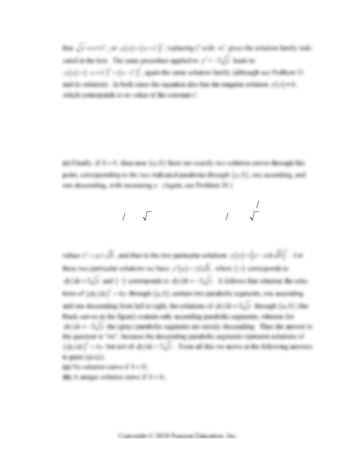
30. The set of solutions of
24
yy
is the
−6 −4 −2 0 2 4 6
−6
4
6
(a, b)
Problem 29c
Section 1.4: Separable Equations and Applications 33
y
y
(a) The given differential equation
24
yy
has no solution curve through the point
,ab if 0b, simply because
20y.
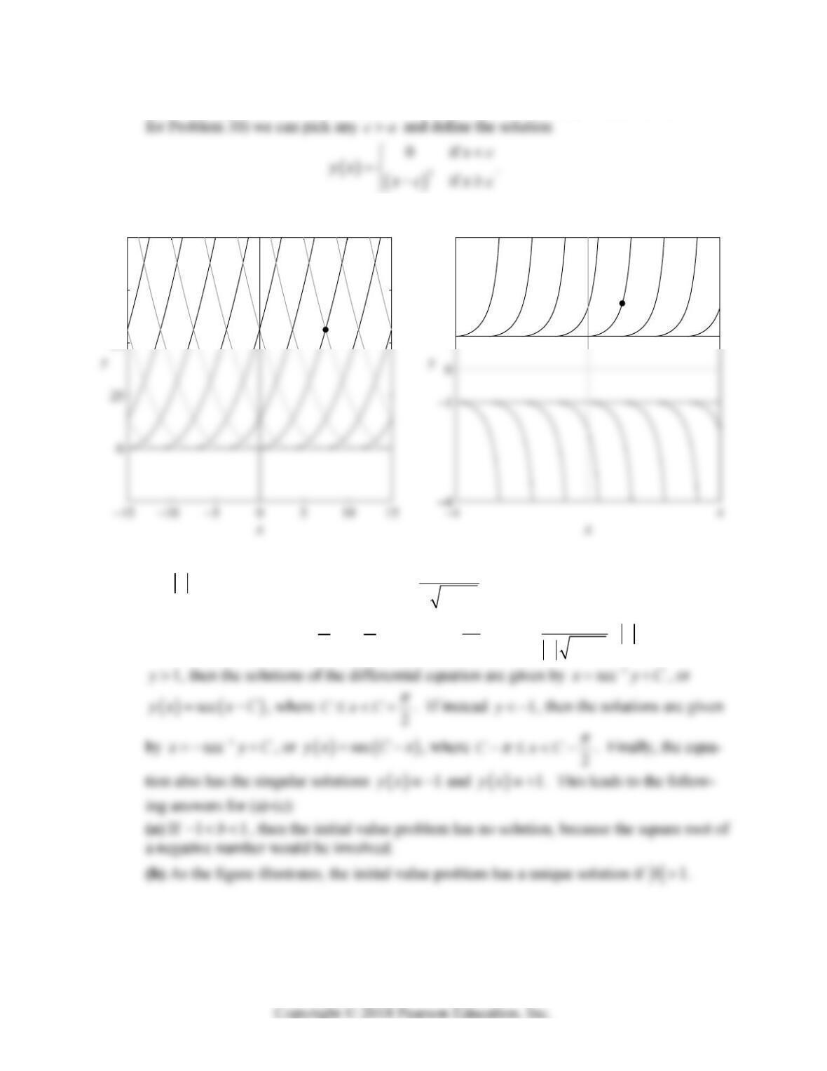
(b) If 0b, then we can combine branches of parabolas with segments along the x-axis
(in the manner of Problems 27-32, Section 1.3) to form infinitely many solution curves
through
,ab that are defined for all x.
31. As noted in Problem 30, the solutions of the differential equation
24d
y
dx
y
consist
of the solutions of 2dy dx y together with those of 2dy dx y , and again we
must have 0y. Imposing the initial condition
ya b, where 0b, upon the general
solution
2
y
xxC found in Problem 30 gives
2
baC , which leads to the two
y
y
y
y
34 Chapter 1: First-Order Differential Equations
(c) Infinitely many solution curves if 0b, because in this case (as noted in the solution
32. For 1y separation of variables gives 2
1
1
dy dx
yy
. We take the inverse secant
function to have range 0, ,
22
, so that 1
2
1
sec
1
dy
dy yy
, 1y. Thus if
50
75
(a, b)
Problem 31
1
4
(a, b)
Problem 32