Section 1.5: Linear First-Order Equations 55
x
x
37. Let
x
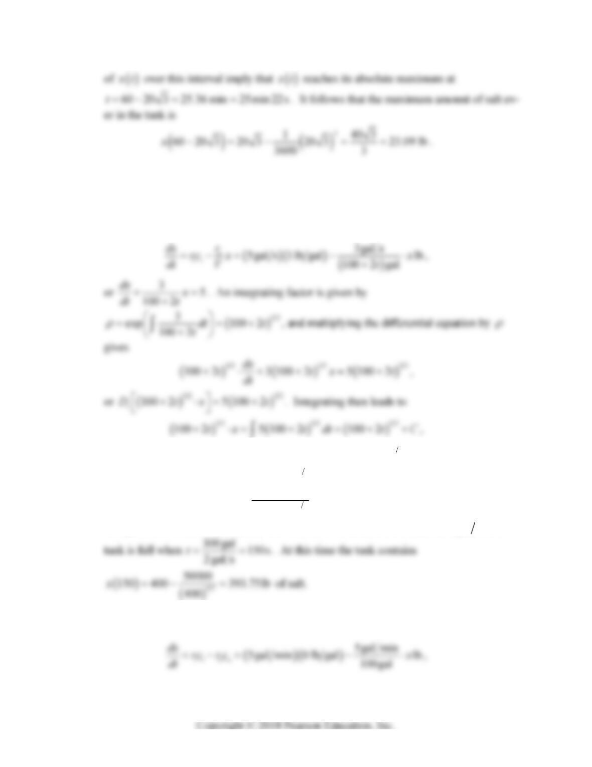
t denote the amount of salt (in lb) after t seconds. Because the volume of liquid
in the tank is increasing by 2 gallon each minute, the volume after t sec is 100 2t gal-
lons. Thus in the notation of Equation (18) of the text, the differential equation for
x
t
is
and thus to the general solution
32
100 2 100 2xt t C t
. The initial condition
050x implies that 32
50 100 100C
, or 50000C , and so the desired particu-
lar solution is
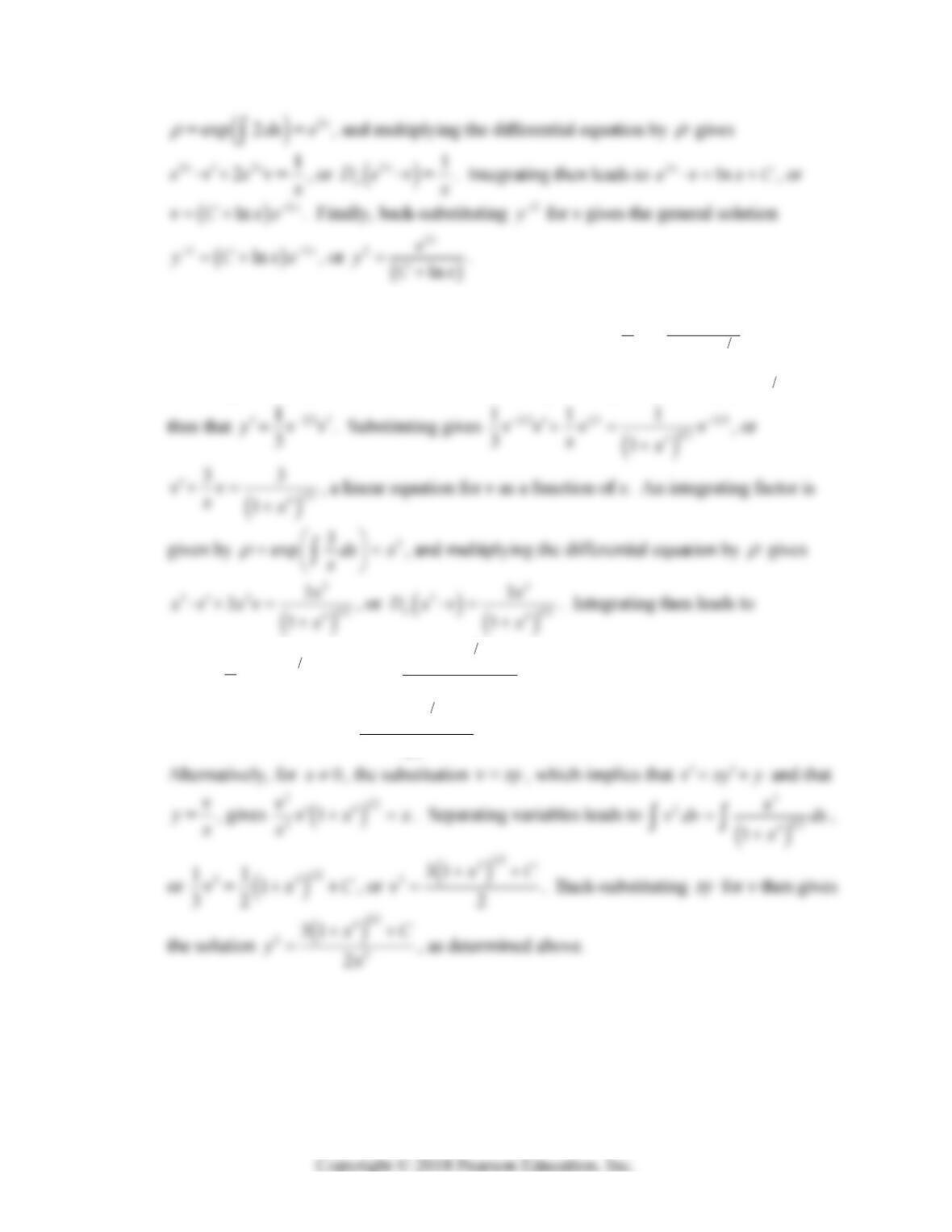
32
50000
100 2 100 2
xt t t
. Finally, because the tank starts out with
300 gallons of excess capacity and the volume of its contents increases at 2gal s, the
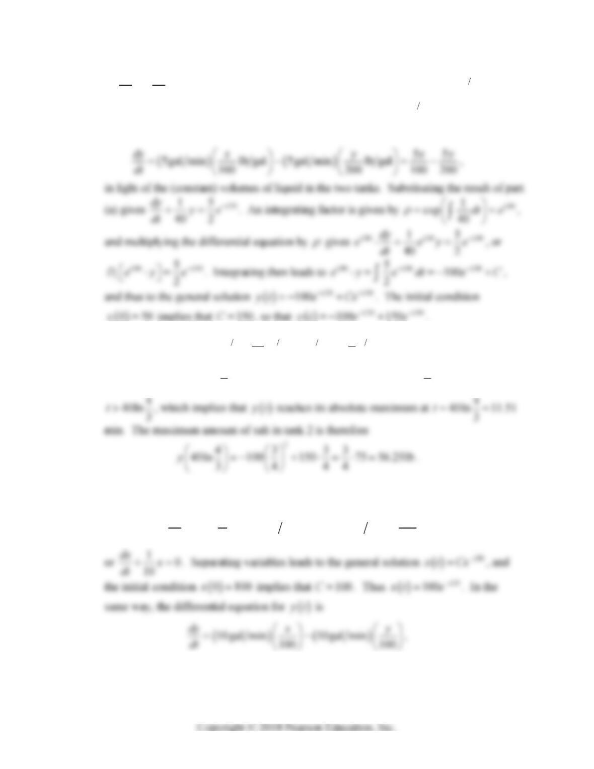
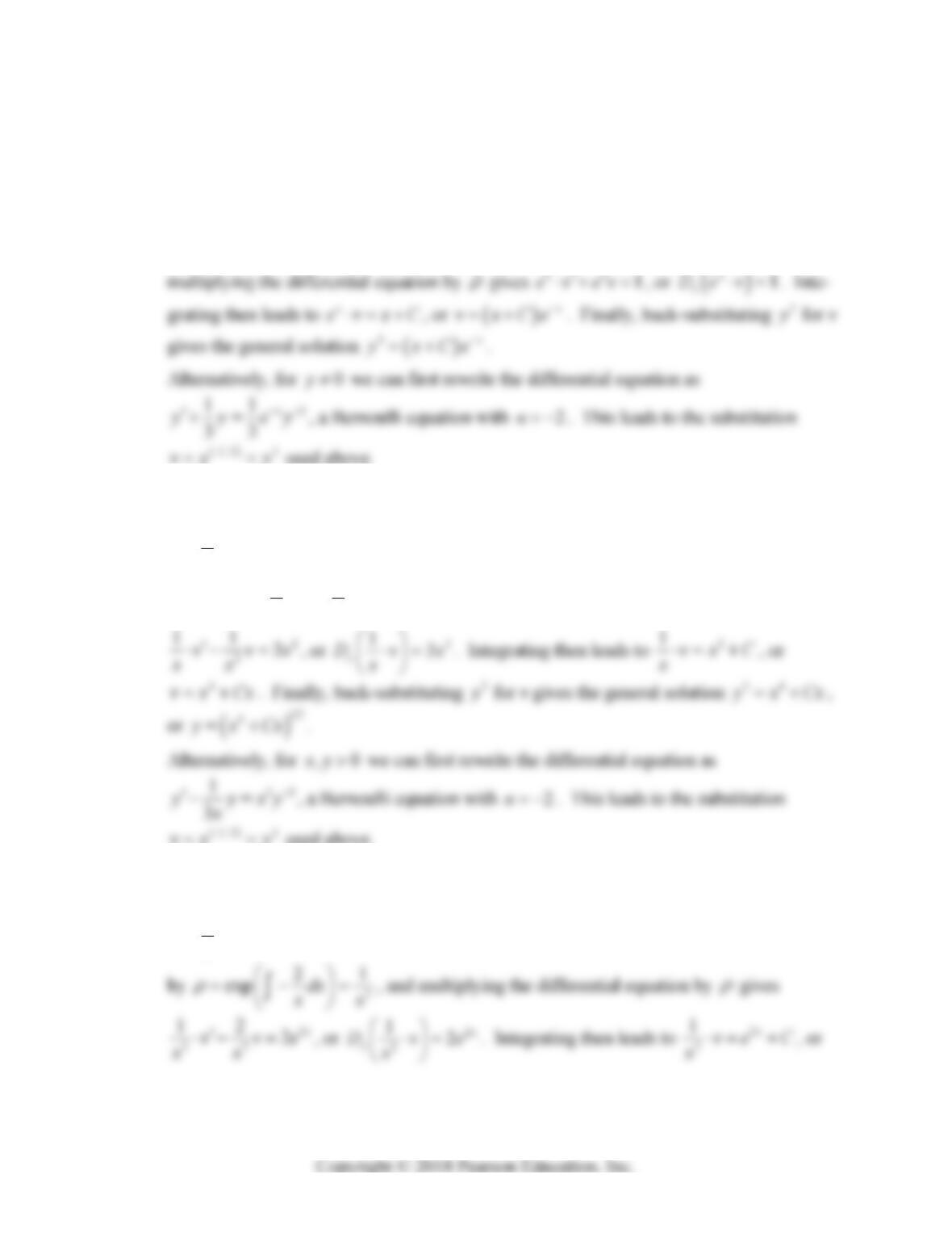
38. (a) In the notation of Equation (16) of the text, the differential equation for
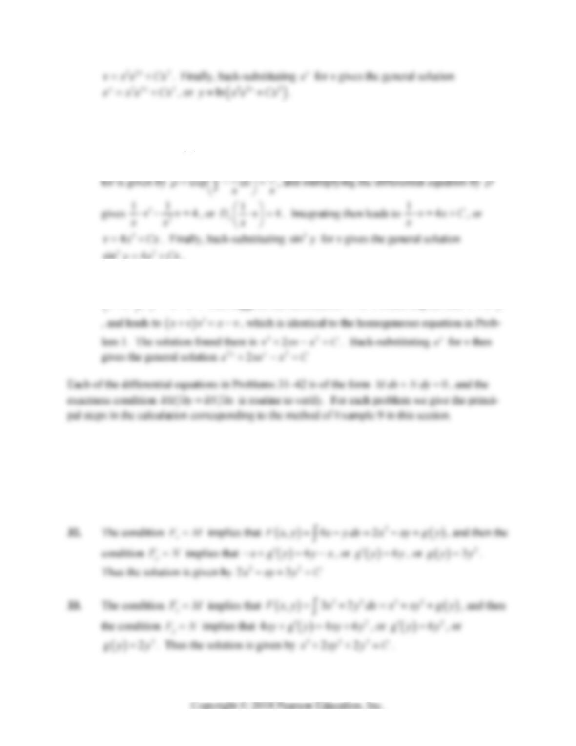
x
t is
56 Chapter 1: First-Order Differential Equations
or 1
20
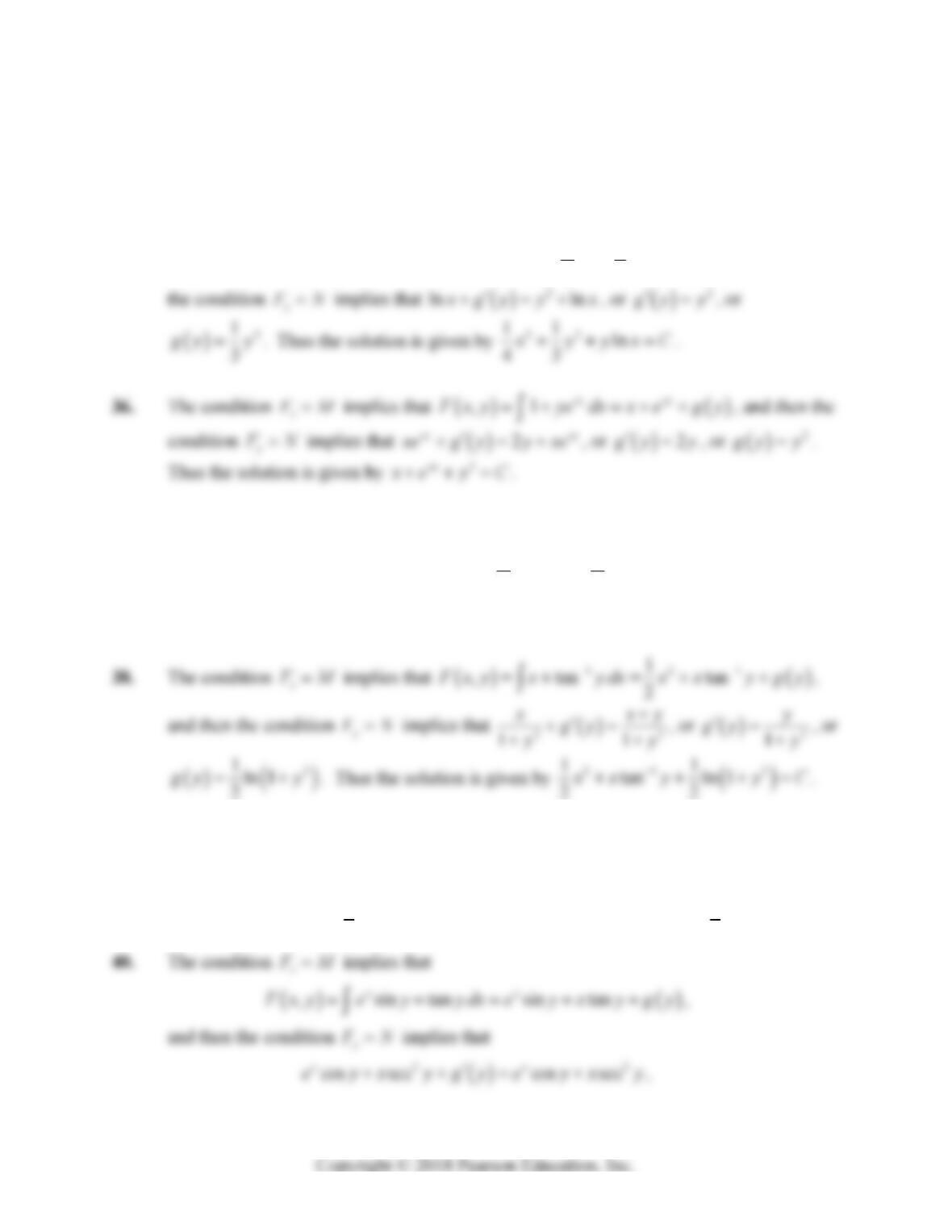
dx
x
dt . Separating variables leads to the general solution
20t
x
tCe
, and the
initial condition
050x implies that 50C. Thus
20
50 t
x
te
.
(b) In the same way, the differential equation for
yt is
(c) By part (b),
20 40 20 40
15 3
551
44
ttt t
yt e e e e
, from which we see that
0yt
when 4
40ln 3
t. Furthermore,
0yt
for 4
040ln
3
t and
0yt
for
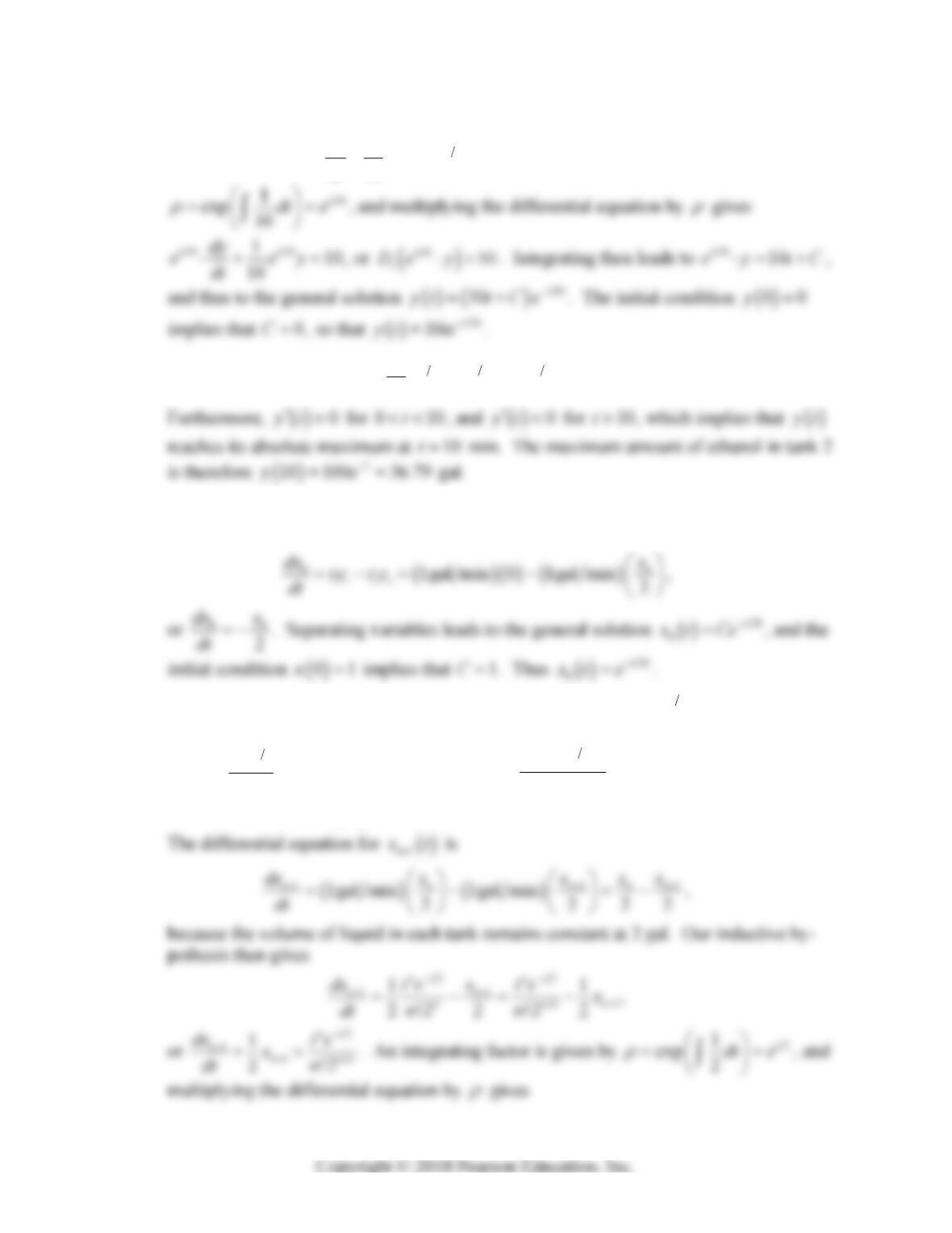
39. (a) In the notation of Equation (18) of the text, the differential equation for
x
t is
10gal min 0 10gal min 100
o
ii
dx r x
rc x
dt V
,
x
x
Section 1.5: Linear First-Order Equations 57
because the volume of liquid in each tank remains constant at 2 gal. Substituting the re-
sult of part (a) gives 10
110
10
t
dy ye
dt
. An integrating factor is given by
(b) By Part (a),
10 10 10
10 10
10
tt t
t
yt e e e t
, which is zero for 10t.
40. (a) In the notation of Equation (16) of the text, the differential equation for
0
x
t is
x
(b) First, when 0n, the proposed formula predicts that
2
0
t
x
te
, which was veri-
fied in part (a). Next, for a fixed positive value of n we assume the inductive hypothesis
2
!2
nt
nn
te
xtn
and seek to show that
12
11
!2
1
nt
nn
te
xtn
; this will prove by mathemat-
ical induction that the proposed formula holds for all 0n.
x
58 Chapter 1: First-Order Differential Equations
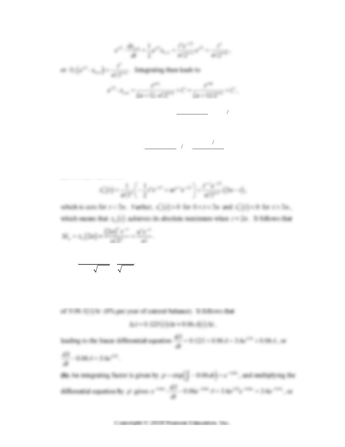
and thus to the general solution
1
2
11
2
1!
n
t
nn
t
x
tCe
n
. The initial condition
100
n
x implies that 0C, so that
11
2
2
111
22
1! 1!
nn
t
t
nnn
tt
e
xt e
nn
,
as desired.
(c) Part (b) implies that
(d) Substituting Sterling’s approximation into the result of part (c) gives
1
22
nn
nnn
e
n
Mne n n
.
41. (a) Between time t and time tt , the amount
At (in thousands of dollars) increases
by a deposit of
0.12St t (12% per year of annual salary) as well as interest earnings
Section 1.5: Linear First-Order Equations 59
42. Since both m and v vary with time, Newton’s second law and the product rule give
dv dm
mv mg
dt dt
. Now since the hailstone is of uniform density 1, its mass
mt
equals its volume
3
3
33
44 4
33 3
k
rkt t
, which means that 32
4
dm kt
dt
. Thus the
velocity
vt of the hailstone satisfies the linear differential equation
43. (a) First we rewrite the differential equation as yx
y
. An integrating factor is given
by
exp 1
x
dx e
, and multiplying the differential equation by
gives
x
xx
y
x
eeye
, or
x
x
x
x
De
y
e
. Integrating (by parts) then leads to
xxxx
x
ey edxxe e C
, and thus to the general solution
1
x
yx x Ce
.
x
60 Chapter 1: First-Order Differential Equations
44. (a) First we rewrite the differential equation as
yy
x
. An integrating factor is given
by
exp 1
x
dx e
, and multiplying the differential equation by
gives
x
xx
y
x
eeye
, or
x
x
x
x
De
y
e
. Integrating (by parts) then leads to
xxxx
x
ey edx xe e C
, and thus to the general solution
1
x
yx x Ce
x
45. The volume of the reservoir (in millions of cubic meters, denoted m-m3) is 2. In the nota-
tion of Equation (18) of the text, the differential equation for
x
t is
3333
0.2 m-m month 10 L m 0.2 m-m month L m
2
o
ii
dx r x
rc x
dt V
,
x
Section 1.5: Linear First-Order Equations 61
46. The volume of the reservoir (in millions of cubic meters, denoted m-m3) is 2. In the nota-
tion of Equation (18) of the text, the differential equation for
x
t is
o
ii
dx r
rc x
dt V
1
10
10
1
and thus to the general solution
10
200 1
20 cos sin
101 10
t
x
tttCe
.
The initial condition
00x implies that 20 102
20 20
101 101
C , and so
x
a pollutant concentration of 3
5L m is reached when
5
2
xt , that is, when
10
20
10 101 102 cos 10sin
101
t
ett
.
62 Chapter 1: First-Order Differential Equations
SECTION 1.6
SUBSTITUTION METHODS AND EXACT EQUATIONS
It is traditional for every elementary differential equations text to include the particular types of
equation that are found in this section. However, no one of them is vitally important solely in its
own right. Their main purpose (at this point in the course) is to familiarize students with the
1. For
0x and 0xy we rewrite the differential equation as
1
1
y
dy x y
x
y
dx x y
x
.
Substituting y
v
x
then gives 1
1
dv v
vx
dx v
, or
2
112
11
dv v v v
xv
dx v v
. Sepa-
x
y
xx
, or 22
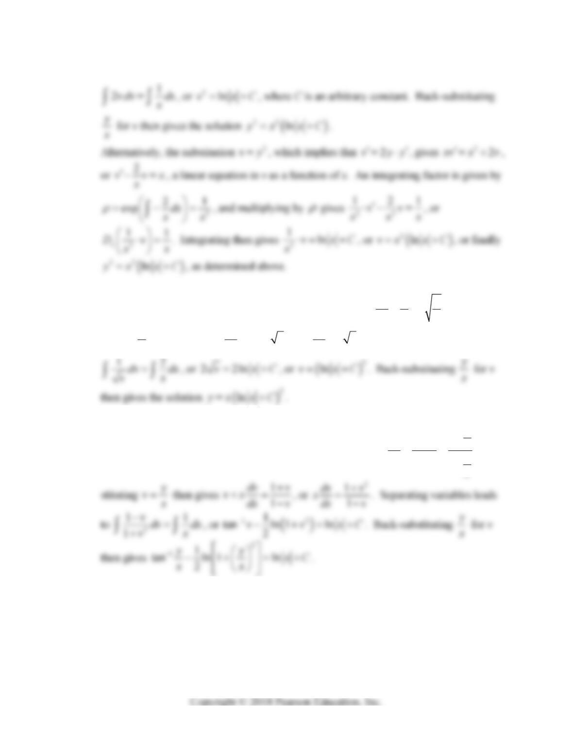
2. For
,0xy we rewrite the differential equation as 1
2
d
y
x
y
dx
y
x
. Substituting y
v
x
then gives 1
2
dv
vx v
dx v
, or 1
2
dv
xdx v
. Separating variables leads to
Section 1.6: Substitution Methods and Exact Equations 63
x
3. For ,
x
y with 0xy we rewrite the differential equation as 2
dy y y
dx x x
. Substitut-
ing
y
v
x
then gives 2
dv
vx v v
dx
, or 2
dv
x
v
dx . Separating variables leads to
y
x
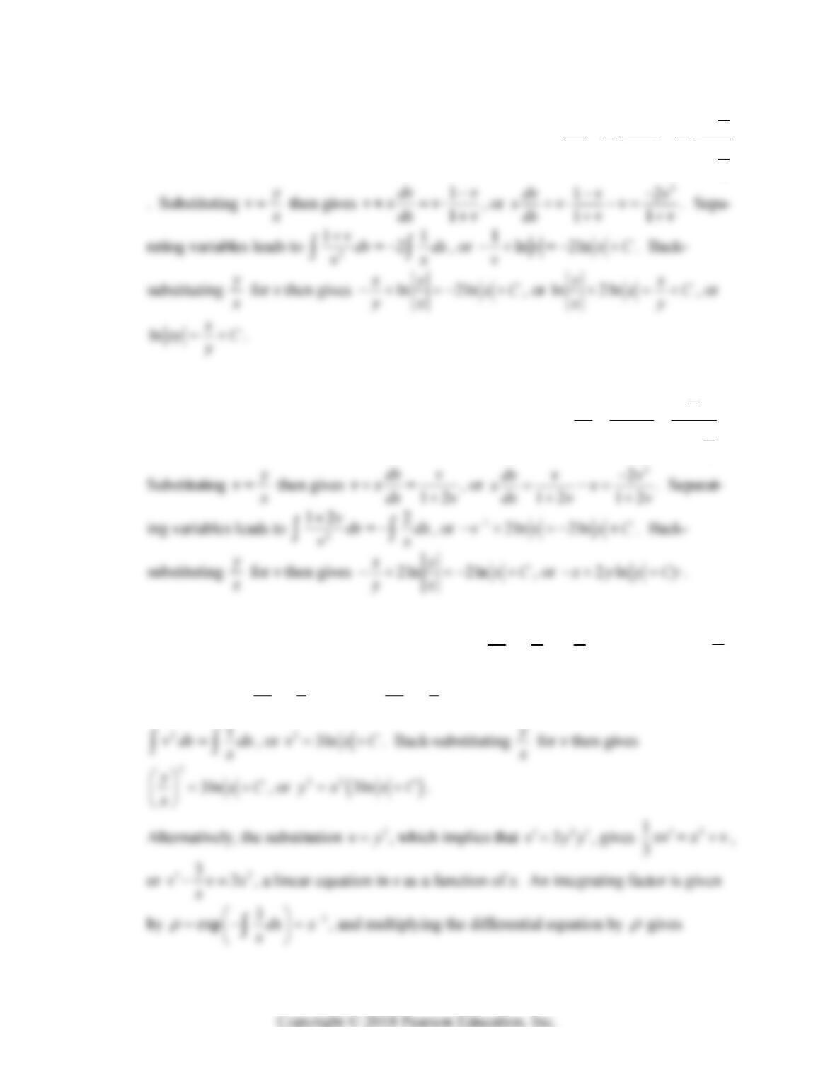
4. For 0x and 0xy we rewrite the differential equation as
1
1
y
dy x y
x
y
dx x y
x
. sub-
y
x
y
x
64 Chapter 1: First-Order Differential Equations
5. For 0x and 0xy we rewrite the differential equation as
1
1
y
dy y x y y
x
y
dx x x y x
x
x
y
x
6. For 20xy and 0x we rewrite the differential equation as 212
y
dy y
x
y
dx x y
x
.
y
x
y
x
x
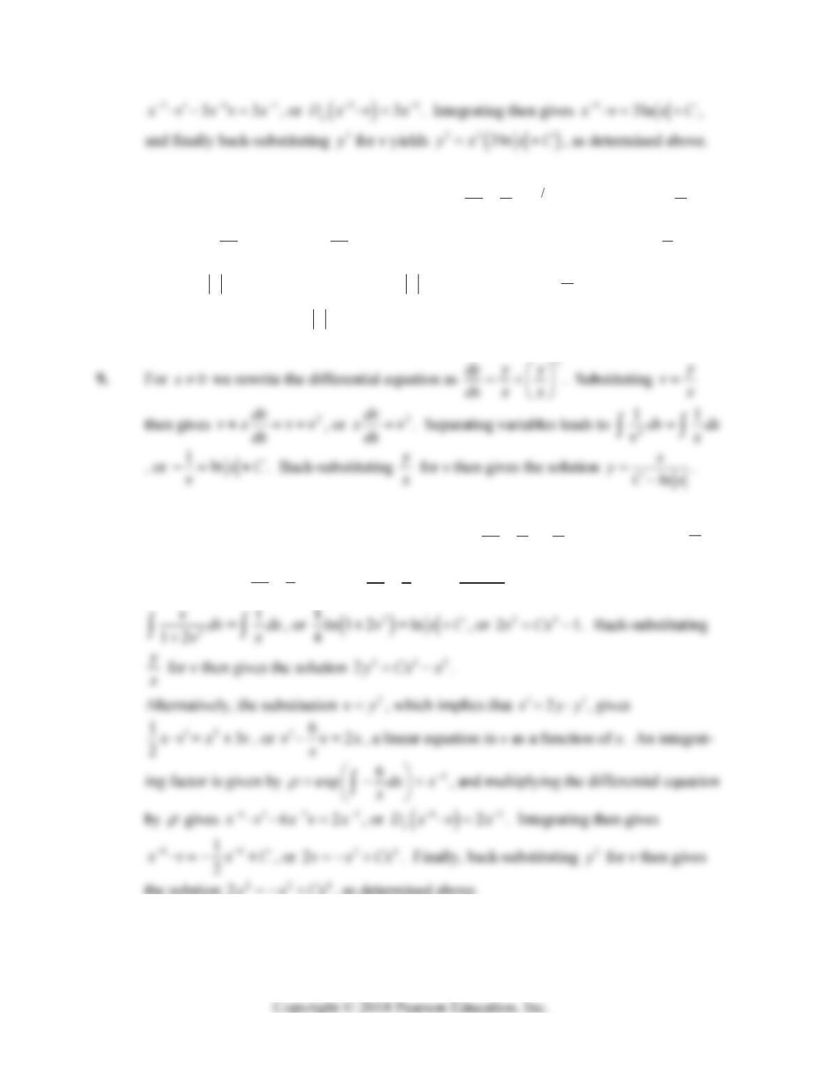
7. For ,0xy we rewrite the differential equation as
2
dy x y
dx y x
. Substituting
y
v
x
then gives
2
1dv
vx v
dx v
, or
2
1dv
xdx v
. Separating variables leads to
x
x
x
Section 1.6: Substitution Methods and Exact Equations 65
y
8. For 0x we rewrite the differential equation as
y
x
dy y e
dx x
. Substituting
y
v
x
then
gives v
dv
vx ve
dx
, or v
dv
x
e
dx . Separating variables leads to 1
v
edv dx
x
, or
ln
v
exC
, that is,
ln lnvCx . Back-substituting
y
x
for v then gives the
solution
ln lnyxC x .
y
x
x
x
y
x
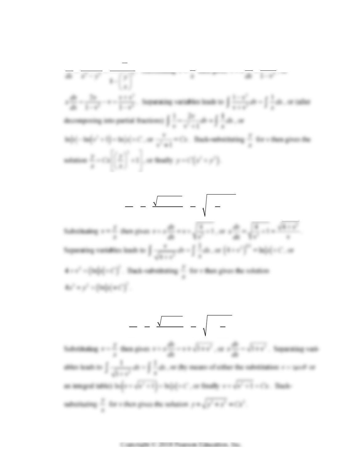
10. For ,0xy we rewrite the differential equation as 3
dy x y
dx y x
. Substituting
y
v
x
then gives 13
dv
vx v
dx v
, or
2
112
2
dv v
xv
dx v v
. Separating variables leads to
y
x
y
x
x
the solution 226
2
y
xCx , as determined above.
66 Chapter 1: First-Order Differential Equations
11. For 22
0xy and 0x we rewrite the differential equation as
x
2
2
y
dy xy
x
y
2
dv v
12. For ,0xy we rewrite the differential equation as
2
22
441
xy
dy y y x
dx x y x y
.
y
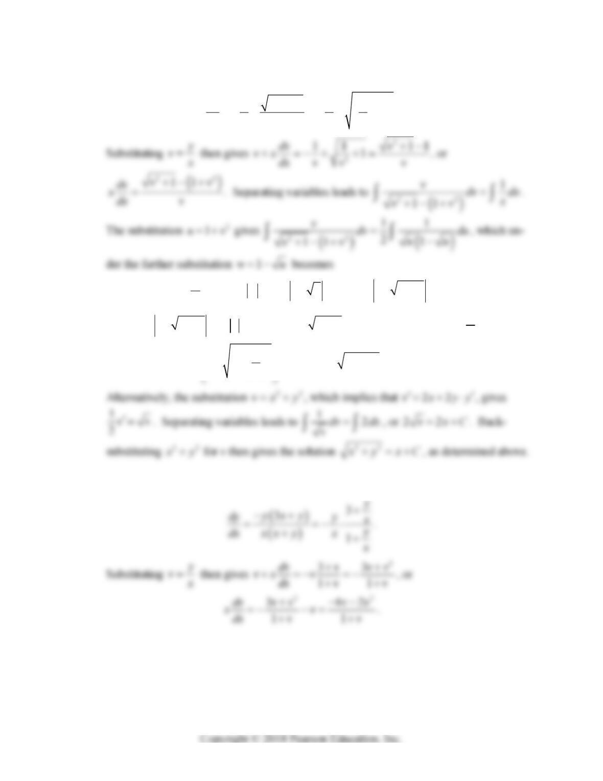
13. For 0x we rewrite the differential equation as
2
22
1
xy
dy y y y
dx x x x x
.
y
y
Section 1.6: Substitution Methods and Exact Equations 67
14. For 0x and 0y we rewrite the differential equation as
2
22
1
xy
dy x x x
dx y y y y
.
y
x
2
1ln ln 1 ln 1 1dw w u C v
w
.
Thus 2
ln 1 1 lnvxC
, or
2
11
x
vC
. Back-substituting
y
x
for v then
gives the solution
2
11y
x
C
x
x
, or 22
x
xyC
.
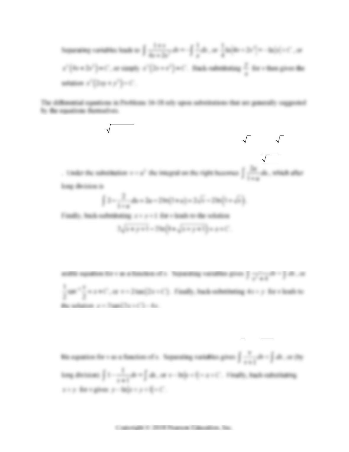
15. For 0x and 0xy we rewrite the differential equation as
y
x
68 Chapter 1: First-Order Differential Equations
16. The expression 1xy suggests the substitution 1vxy, which implies that
1yvx, and thus that 1yv
. Substituting gives 1vv
, or 1vv
, a
separable equation for v as a function of x. Separating variables gives 1
1dv dx
v
x
17. The expression 4
x
y suggests the substitution 4vxy, which implies that
4yv x , and thus that 4yv
. Substituting gives 2
4vv
, or 24vv
, a sep-
x
18. The expression
xy
suggests the substitution vx
y
, which implies that yvx,
and thus that 1yv
. Substituting gives
11vv
, or 11
1v
vvv
, a separa-
Section 1.6: Substitution Methods and Exact Equations 69
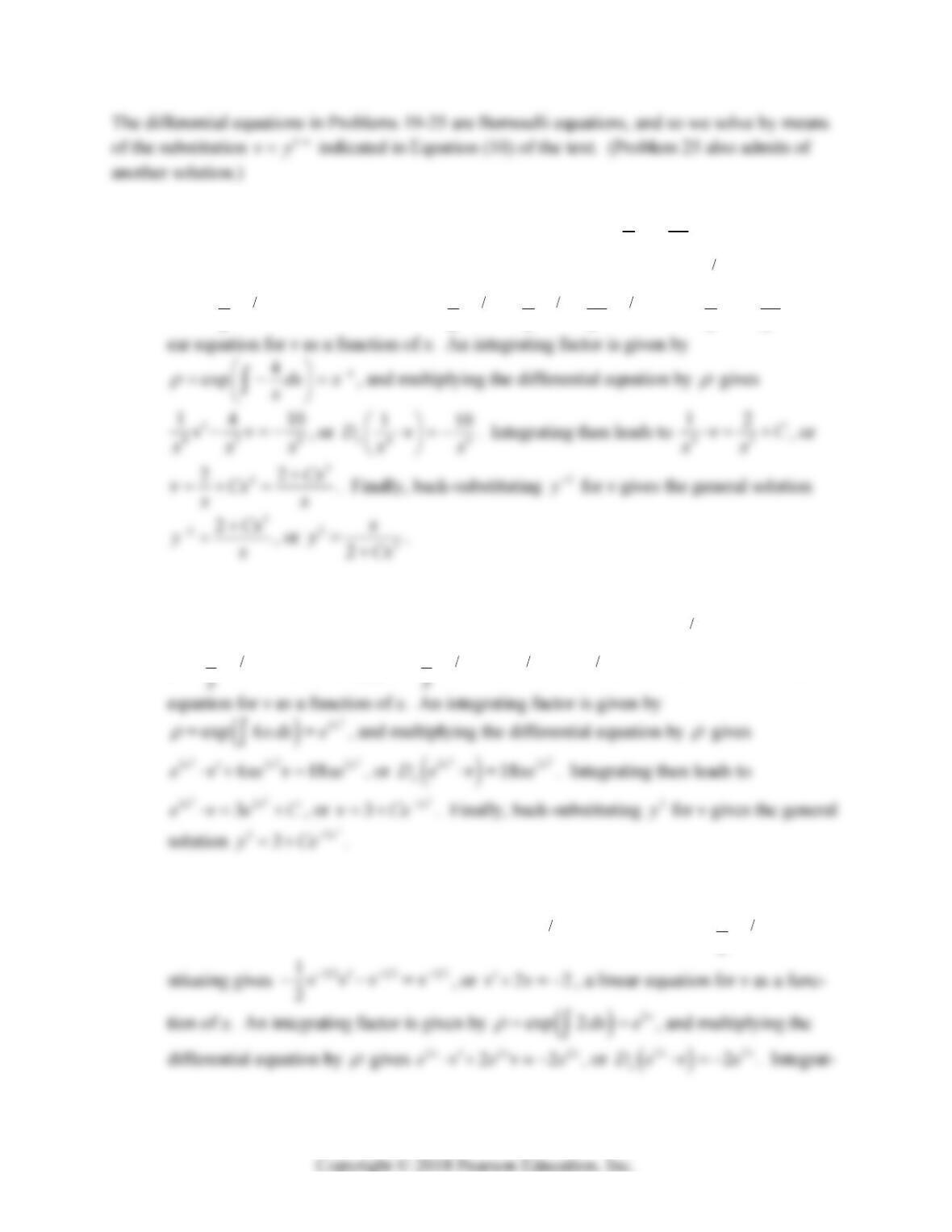
19. We first rewrite the differential equation for ,0xy as 3
2
25
y
yy
xx
, a Bernoulli
equation with 3n. The substitution 13 2
vy y
implies that 12
y
v
and thus that
32
1
2
y
vv
. Substituting gives 32 12 32
2
125
2vv v v
xx
, or 2
410
vv
x
x
, a lin-
x
y
x
20. We first rewrite the differential equation for 0y as 2
26
y
xy xy
, a Bernoulli equa-
tion with 2n . The substitution
12 3
vy y
implies that 13
y
v and thus that
23
1
y
y
vv
. Substituting gives 23 13 23
126
, or 618vxv x
, a linear
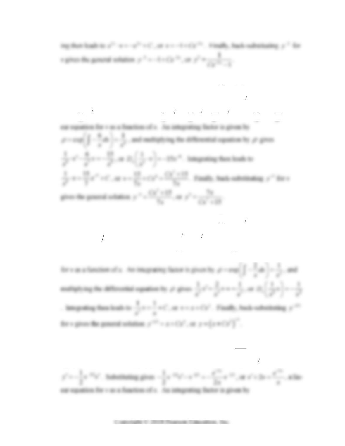
21. We first rewrite the differential equation as 3
y
yy
, a Bernoulli equation with 3n.
The substitution 13 2
vy y
implies that 12
y
v
and thus that 32
1
2
yvv
. Sub-
70 Chapter 1: First-Order Differential Equations
y
y
22. We first rewrite the differential equation for 0x as 4
2
25
y
yy
xx
, a Bernoulli equa-
tion with 4n. The substitution 14 3
vy y
implies that 13
y
v
and thus that
43
1
y
yvv
. Substituting gives 43 13 43
2
125
, or 2
615
vv
, a lin-
23. We first rewrite the differential equation for 0x as 43
63
y
yy
x
, a Bernoulli equa-
tion with 43n. The substitution
143 13
vy y
implies that 3
y
v
and thus that
4
3
y
vv
. Substituting gives 434
6
33vv v v
x
, or 21vv
x
, a linear equation
y
y
24. We first rewrite the differential equation for 0x as
2
3
2
x
e
yy y
x
, a Bernoulli
equation with 3n. The substitution 13 2
vy y
implies that 12
y
v
, and thus that
y
Section 1.6: Substitution Methods and Exact Equations 71
x
x
25. We first rewrite the differential equation for ,0xy as
2
12
4
11
1
yy y
xx
, a Ber-
noulli equation with 2n . The substitution
12 3
vy y
implies that 13
y
v and
12
34
31
2
x
vxC , or
12
4
3
31
2
x
C
vx
. Finally, back-substituting 3
y
for v gives
the general solution
12
4
3
3
31
2
x
C
yx
.
x
x
x
72 Chapter 1: First-Order Differential Equations
As with Problems 16-18, the differential equations in Problems 26-30 rely upon substitutions that
are generally suggested by the equations themselves. Two of these equations are also Bernoulli
equations.
26. The substitution 3
vy, which implies that 2
3vyy
, gives
x
vve
, a linear equa-
tion for v as a function of x. An integrating factor is given by
exp 1
x
dx e
, and
x
x
27. The substitution 3
vy, which implies that 2
3vyy
, gives 4
3
x
vv x
, or (for 0x)
3
13vvx
x
, a linear equation for v as a function of x. An integrating factor is given by
11
exp dx
x
x
, and multiplying the differential equation by
gives
vy y
used above.
28. The substitution y
ve, which implies that y
vey
, gives
32
2
x
x
vvxe
, or
22
22
x
vvxe
x
, a linear equation for v as a function of x. An integrating factor is given
x
x
Section 1.6: Substitution Methods and Exact Equations 73
29. The substitution 2
sinvy, which implies that
2sin cosvyyy
, gives 2
4
x
vxv
,
or (for 0x) 14vvx
x
, a linear equation for v as a function of x. An integrating fac-
30. It is easiest first to multiply each side of the given equation by y
e, giving
yy y
x
eey xe
. This suggests the substitution y
ve, which implies that y
vey
x
31. The condition x
FM implies that
2
,23 3Fxy x ydx x xy gy
, and then
the condition y
FN implies that
332
x
gy x y
, or
2gy y
, or
2
gy y.
Thus the solution is given by 22
3
x
xy y C.
x
x
x
74 Chapter 1: First-Order Differential Equations
34. The condition x
FM implies that
22 322
,23Fxy xy xdx x xy gy
, and
then the condition y
FN implies that
223
224
x
ygy xy y
, or
3
4gy y
, or
4
gy y. Thus the solution is given by 322 4
x
xy y C.
35. The condition x
FM implies that
34
1
,ln
4
y
Fxy x dx x y x gy
x
, and then
x
g
x
x
x
37. The condition x
FM implies that
,coslnsinlnFxy x ydx x x y gy
,
and then the condition y
FN implies that
y
xx
gy e
yy
, or
y
gy e
, or
y
gy e. Thus the solution is given by sin ln y
x
xye C.
g
x
39. The condition x
FM implies that
23 4 33 4
,3Fxy xy ydx xy xy gy
, and
then the condition y
FN implies that
32 3 32 4 3
34 3 4
x
yxygyxyyxy
, or
4
gy y
, or
5
1
5
g
yy. Thus the solution is given by 33 4 5
1
5
x
yxy yC
.