Section 2.5: A Closer Look at the Euler Method 155
% ‘impeuler’, ‘rk’ (Runge-Kutta), ‘ode23’, ‘ode45’.
% Results are saved at the endPoints of n subintervals,
% that is, in steps of length h = (b – t0)/n. The
% result t is an (n+1)-column vector from b to t1,
% while y is a matrix with n+1 rows (one for each
% t-value) and one column for each dependent variable.
To use the improved Euler method, we call as ‘method’ the following function.
function [t,y] = impeuler(yp, t0,t1, y0)
%
% [t,y] = impeuler(yp, t0,t1, y0)
% Takes one improved Euler step for
%
% y’ = yprime( t,y ),
%
29. Here our differential equation is described by the MATLAB function
function vp = vpbolt1(t,v)
vp = -0.04*v – 9.8;
Then the commands
156 Chapter 2: Mathematical Models and Numerical Methods
generate the table
t with
50n
with
100n actual v
0 49.0000 49.0000 49.0000
1 37.4722 37.4721 37.4721
2 26.3964 26.3963 26.3962
We notice first that the final two columns agree to 3 decimal places (each difference
being less than 0.0005). Scanning the 100n column for sign changes, we suspect that
100v (at the bolt’s apex) occurs just after 4.5sect. Then interpolation between
4.5t and 4.6t in the table
[t2(40:51),v2(40:51)]
3.9000 6.5345
4.0000 5.5304
4.1000 4.5303
Section 2.5: A Closer Look at the Euler Method 157
9.4000 -43.1387
9.5000 -43.9445
gives the impact velocity
9.41 43.22 m sv .
30. Now our differential equation is described by the MATLAB function
function vp = vpbolt2(t,v)
vp = -0.0011*v.*abs(v) – 9.8;
Then the commands
generate the table
t with 100n with 200n
0 49.0000 49.0000
1 37.1547 37.1547
2 26.2428 26.2429
We notice first that the final two columns agree to 2 decimal places (each difference
being less than 0.005). Scanning the 200n column for sign changes, we suspect that
158 Chapter 2: Mathematical Models and Numerical Methods
[t2(91:101),v2(91:101)]
4.5000 1.0964
4.5500 0.6063
4.6000 0.1163
4.6500 -0.3737
indicates that 4.61T at the bolt’s apex. Finally, interpolation in
[t2(189:190),v2(189:190)]
9.4000 -43.4052
SECTION 2.6
THE RUNGE-KUTTA METHOD
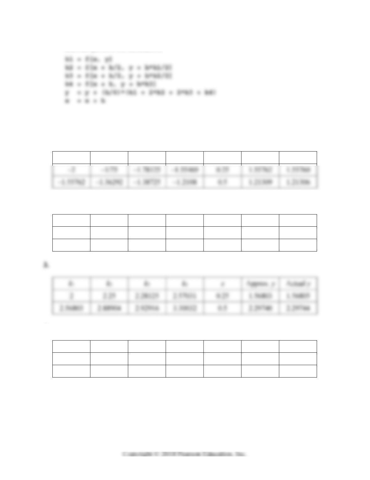
Each problem can be solved with a “template” of computations like those listed in Problem 1.
We include a table showing the slope values 1
k, 2
k, 3
k, 4
k and the xy-values at the ends of two
successive steps of size 0.25h.
Section 2.6: The Runge-Kutta Method 159
and then perform the calculations
in turn. Here we are using Mathematica notation that translates transparently to standard
mathematical notation describing the corresponding manual computations. A repetition
of this same block of calculations carries out a second step of size 0.25h. The
following table lists the intermediate and final results obtained in these two steps.
k1 k2 k3 k4 x Approx. y Actual y
2.
k1 k2 k3 k4 x Approx. y Actual y
1 1.25 1.3125 1.65625 0.25 0.82422 0.82436
1.64844 2.06055 2.16357 2.73022 0.5 1.35867 1.35914
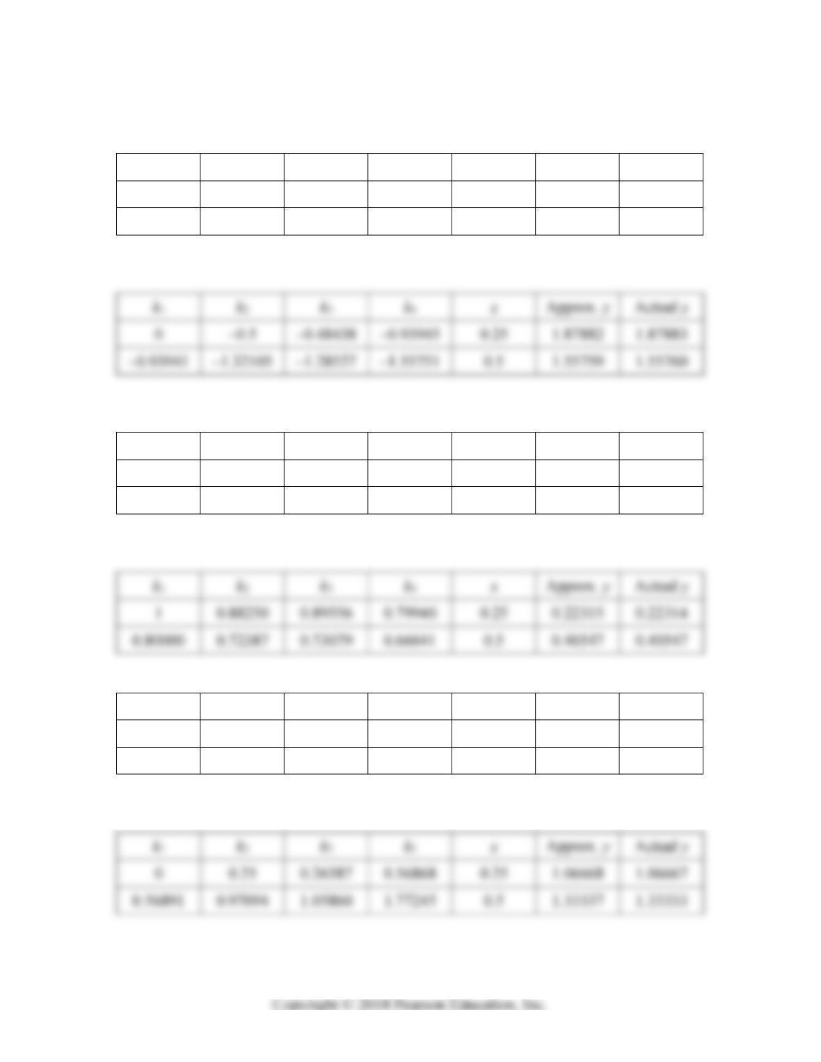
4.
k1 k2 k3 k4 x Approx. y Actual y
–1 –0.75 –0.78128 –55469 0.25 0.80762 0.80760
–0.55762 –0.36292 –0.38725 –0.21080 0.5 0.71309 0.71306
160 Chapter 2: Mathematical Models and Numerical Methods
5.
k1 k2 k3 k4 x Approx. y Actual y
0 –0.125 –0.14063 –0.28516 0.25 0.96598 0.96597
–28402 –0.44452 –0.46458 –0.65016 0.5 0.85130 0.85128
6.
7.
k1 k2 k3 k4 x Approx. y Actual y
0 –0.14063 –0.13980 –0.55595 0.25 2.95347 2.95349
–0.55378 –1.21679 –1.18183 –1.99351 0.5 2.6475 2.64749
8.
9.
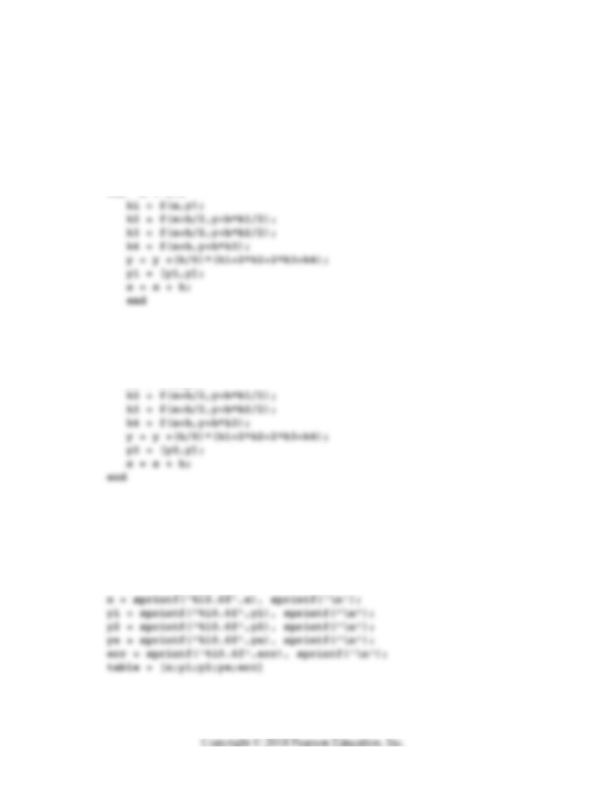
k1 k2 k3 k4 x Approx. y Actual y
0.5 0.53223 0.53437 0.57126 0.25 1.13352 1.13352
0.57122 0.61296 0.61611 0.66444 0.5 1.28743 1.28743
10.
Section 2.6: The Runge-Kutta Method 161
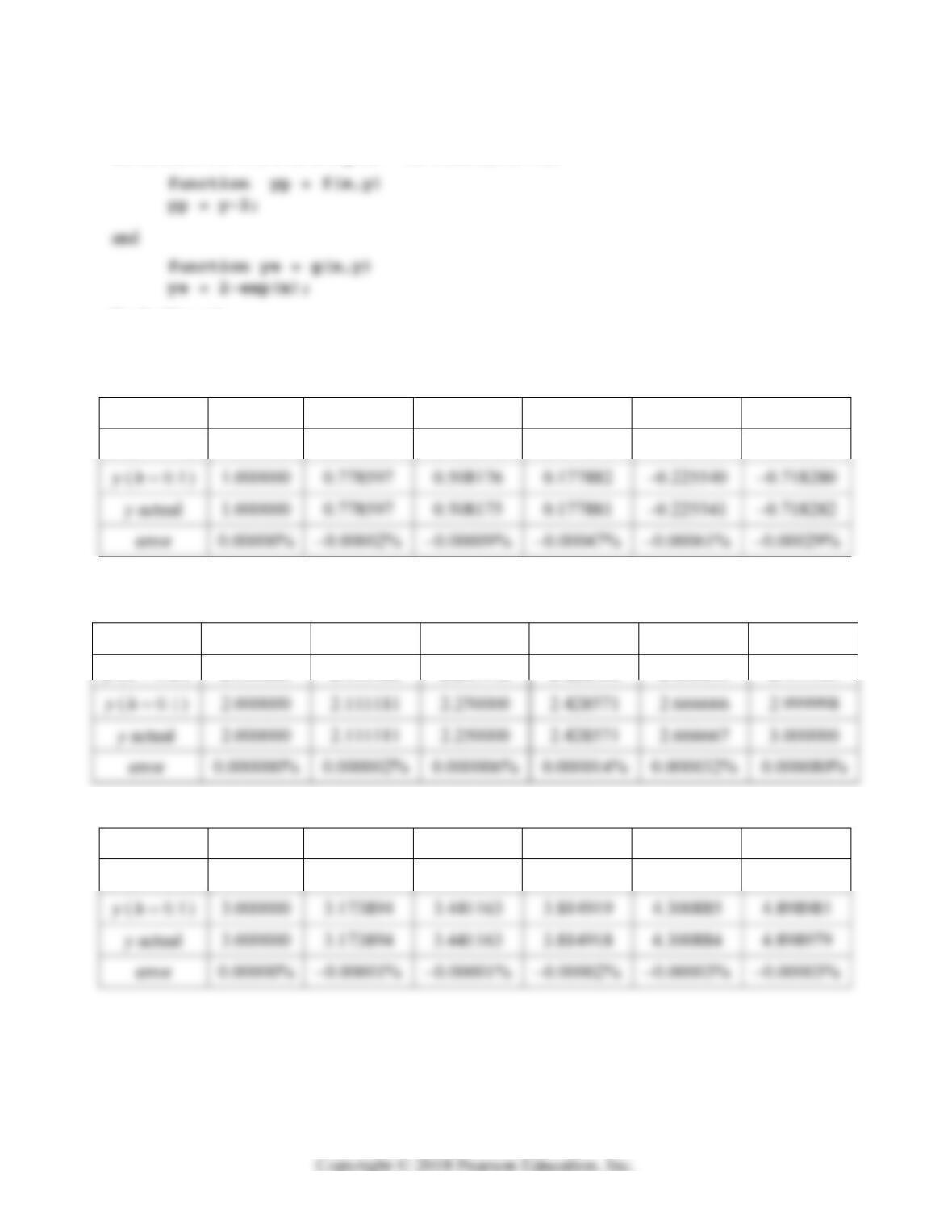
The results given below for Problems 11–16 were computed using the following MATLAB
script.
% Section 2.6, Problems 11-16
x0 = 0; y0 = 1;
% first run:
h = 0.2;
x = x0; y = y0; y1 = y0;
for n = 1:5
% second run:
h = 0.1;
x = x0; y = y0; y2 = y0;
for n = 1:10
k1 = f(x,y);
% exact values
x = x0 : 0.2 : x0+1;
ye = g(x);
% display table
y2 = y2(1:2:11);
err = 100*(ye-y2)./ye;
162 Chapter 2: Mathematical Models and Numerical Methods
For each problem the differential equation
,yfxy
and the known exact solution
ygx
are stored in the files f.m and g.m — for instance, the files
for Problem 11.
11.
x 0.0 0.2 0.4 0.6 0.8 1.0
y ( 0.2h) 1.000000 0.778600 0.508182 0.177894 –0.225521 –0.718251
12.
x 0.0 0.2 0.4 0.6 0.8 1.0
y ( 0.2h) 2.000000 2.111110 2.249998 2.428566 2.666653 2.999963
13.
x 1.0 1.2 1.4 1.6 1.8 2.0
y ( 0.2h) 3.000000 3.173896 3.441170 3.814932 4.300904 4.899004
14.
x 1.0 1.2 1.4 1.6 1.8 2.0
y ( 0.2h) 1.000000 1.222957 1.507040 1.886667 2.425586 3.257946
15.
x 2.0 2.2 2.4 2.6 2.9 3.0
y ( 0.2h) 3.000000 3.026448 3.094447 3.191719 3.310207 3.444447
16.
x 2.0 2.2 2.4 2.6 2.9 3.0
y ( 0.2h) 3.000000 4.243067 5.361409 6.478634 7.634049 8.845150
17.
Value of h Estimated value of
1y
0.2 0.350258
164 Chapter 2: Mathematical Models and Numerical Methods
The table of numerical results is
x y with 0.2h y with 0.1h y with 0.05h y with 0.025h
0.0 0.000000 0.000000 0.000000 0.000000
0.2 0.002667 0.002667 0.002667 0.002667
18.
Value of h Estimated value of
2y
0.2 1.679513
19.
Value of h Estimated value of
2y
0.2 1.679459
20.
Value of h Estimated value of
2y
0.2 –1.259990
Section 2.6: The Runge-Kutta Method 165
21.
Value of h Estimated value of
2y
0.2 2.872467
22.
Value of h Estimated value of
2y
0.2 7.326761
23.
Value of h Estimated value of
1y
0.2 1.230735
24.
Value of h Estimated value of
1y
0.2 1.000000
166 Chapter 2: Mathematical Models and Numerical Methods
25. Here
,321.6
f
tv v and 00t, 00v. With 0.1h, 10 iterations of
12 1
11
,,
22
nn n n
kftv kft hv hk
26. Here
2
, 0.0225 0.003
f
tP P P
and 00t, 025P. With 6h, 10 iterations of
12 1
11
,,
22
nn n n
kftP kft hP hk
27. Here
22
,1fxy x y
and 00x, 00y. The following table gives the
approximate values for the successive step sizes h and corresponding numbers n of steps.
It appears likely that
2 1.00445y rounded off accurate to 5 decimal places.
h 1 0.1 0.01 0.001
Section 2.6: The Runge-Kutta Method 167
28. Here
2
1
,2
f
xy x y and 02x , 00y. The following table gives the approximate
values for the successive step sizes h and corresponding numbers n of steps. It appears
likely that
2 1.46331y rounded off accurate to 5 decimal places.
h 1 0.1 0.01 0.001
function [t,y] = rk(yp, t0,t1, y0)
% [t, y] = rk(yp, t0, t1, y0)
% Takes one Runge-Kutta step for
%
% y’ = yp( t,y ),
29. Here our differential equation is described by the MATLAB function
function vp = vpbolt1(t,v)
vp = -0.04*v – 9.8;
Then the commands
n = 100;
168 Chapter 2: Mathematical Models and Numerical Methods
generate the table
t with 100n with 200n actual v
0 49.0000 49.0000 49.0000
1 37.4721 37.4721 37.4721
We notice first that the final three columns agree to the 4 displayed decimal places. Scanning the
last column for sign changes in v, we suspect that 0v (at the bolt’s apex) occurs just after
4.5sect. Then interpolation between 4.55t and 4.60t in the table
[t2(91:95),v(91:95)]
4.5000 0.5694
4.5500 0.0788
indicates that 4.56t at the bolt’s apex. Now the commands
y = zeros(n+1,1);
h = 10/n;
for j = 2:n+1
Section 2.6: The Runge-Kutta Method 169
t approx. y actual y
0 0 0
1 43.1974 43.1976
2 75.0945 75.0949
3 96.1342 96.1348
We see at least 2-decimal place agreement between approximate and actual values of y.
Finally, interpolation between 9t and 10t here suggests that 0y just after
9.4t. Then interpolation between 9.40t and 9.45t in the table
[t2(187:191),y(187:191)]
9.3000 4.7448
30. Now our differential equation is described by the MATLAB function
function vp = vpbolt2(t,v)
vp = -0.0011*v.*abs(v) – 9.8;
Then the commands
170 Chapter 2: Mathematical Models and Numerical Methods
[t, v1(1:n/20:1+n/2), v(1:n/10:n+1), ve]
generate the table
t with 200n with 400n actual v
0 49.0000 49.0000 49.0000
1 37.1548 37.1548 37.1547
2 26.2430 26.2430 26.2429
We notice first that the final three columns almost agree to the 4 displayed decimal
places. Scanning the last column for sign changes in v, we suspect that 0v (at the
bolt’s apex) occurs just after 4.6sect. Then interpolation between 4.600t and
4.625t in the table
[t2(185:189),v(185:189)]
4.6000 0.1165
indicates that 4.61t at the bolt’s apex. Now the commands
y = zeros(n+1,1);
h = 10/n;
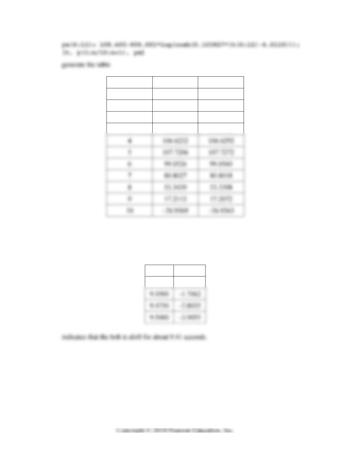
Section 2.6: The Runge-Kutta Method 171
t Approx. y Actual y
0 0 0.0001
1 42.9881 42.9841
2 74.6217 74.6197
3 95.6719 95.6742
We see almost 2-decimal place agreement between approximate and actual values of y.
Finally, interpolation between 9t and 10t here suggests that 0y just after
9.4t. Then interpolation between 9.400t and 9.425t in the table
[t2(377:381),y(377:381)]
9.4000 0.4740
9.4250 –0.6137
CHAPTER 3
LINEAR SYSTEMS AND MATRICES
SECTION 3.1
INTRODUCTION TO LINEAR SYSTEMS
This initial section takes account of the fact that some students remember only hazily the method of
elimination for 22and 33 systems. Moreover, high school algebra courses generally
emphasize only the case in which a unique solution exists. Here we treat on an equal footing the
other two cases — in which either no solution exists or infinitely many solutions exist.
1. Subtraction of twice the first equation from the second equation gives 510,y so
y = 2, and it follows that x = 3.
4. Subtraction of 6/5 times the first equation from the second equation gives 11 44 ,
55
y
so y = 4, and it follows that x = 5.
5. Subtraction of twice the first equation from the second equation gives 01, so no
solution exists.
174 Chapter 3: Linear Systems and Matrices
10. Subtraction of twice the first equation from the second equation gives 3 5.yz
11. First we interchange the first and second equations. Then subtraction of twice the new
first equation from the new second equation gives 7,yz and subtraction of three
12. First we interchange the first and third equations. Then subtraction of twice the new first
equation from the second equation gives 7 3 36,yz and subtraction of twice the
13. First we subtract the second equation from the first equation to get the new first equation
230.xyz Then subtraction of twice the new first equation from the second
equation gives 3 2 0,yz and subtraction of twice the new first equation from the
third equation gives 2 0.yz Solution of these latter two equations gives
0, 0.yz Finally substitution in the (new) first equation gives x = 0 also.
15. Subtraction of the first equation from the second equation gives 4 2.yz
Subtraction of three times the first equation from the third equation gives (after division
by 2) 4 5 / 2.yz These latter two equations obviously are inconsistent, so the
original system has no solution.