FIND: Lagrangian expression =0
(,)VVVt
where 0
V is car velocity at time =0t and 0x=.
SOLUTION: The condition =0
VV
at =0x gives
or
×
=−=
1293.1
ln 1 1.0
0.1 88.5
B
so
=+
0(1 e )
2
x
V
V
To find =0
(,)VVVt
, we note that
Carrying out the integration gives
DISCUSSION: Equation(1) can be written as
0
22
ln 1
x
x
e
tVe
=
+
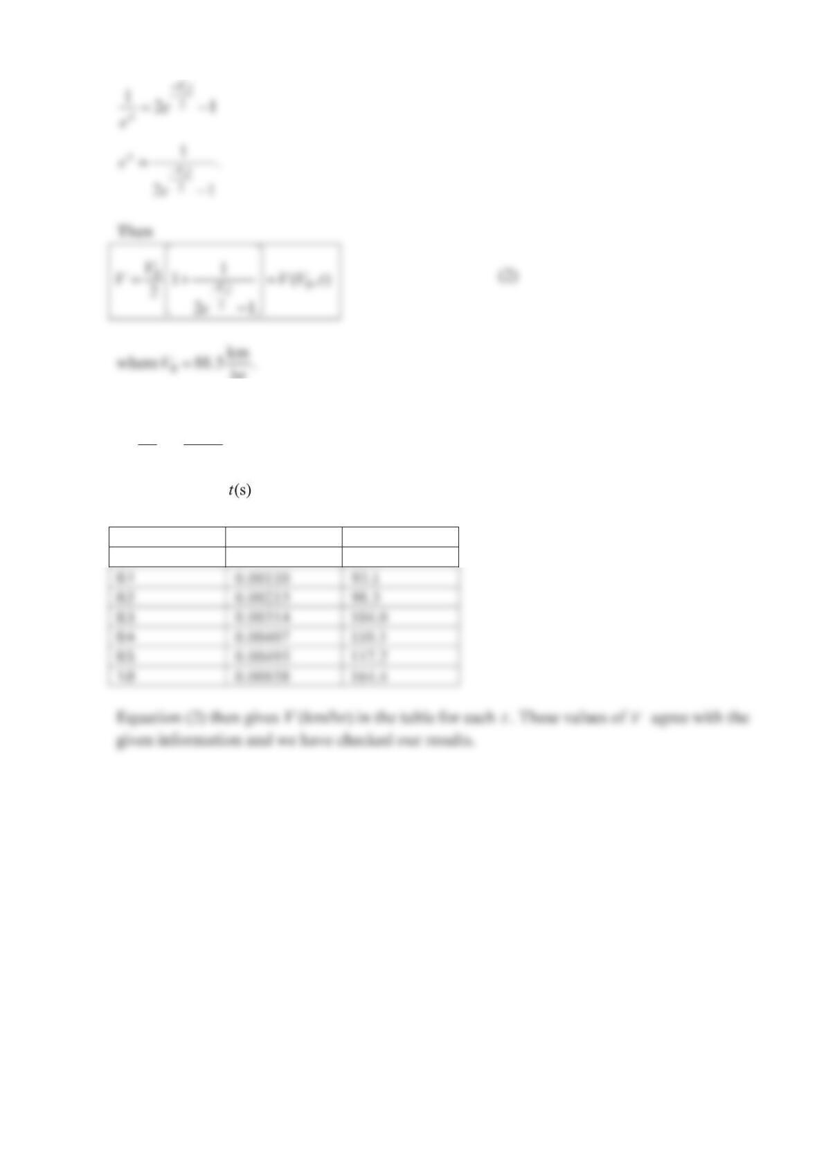
which gives the in the following table for each x.
x
(km) t (s) V (km/hr)
0 088.5
Problem 4.17
A tornado has the following velocity components in polar coordinates:
=− 1
r
C
Vr and
θ
=− 2
C
Vr.
Note that the air is spiraling inward. Find an equation for the streamlines. r and
θ
are
polar coordinates.
Solution 4.17
GIVEN: Tornado with velocity components
=− 1
r
C
Vr and
θ
=− 2
C
Vr.
FIND: Equation for the streamline of the air.
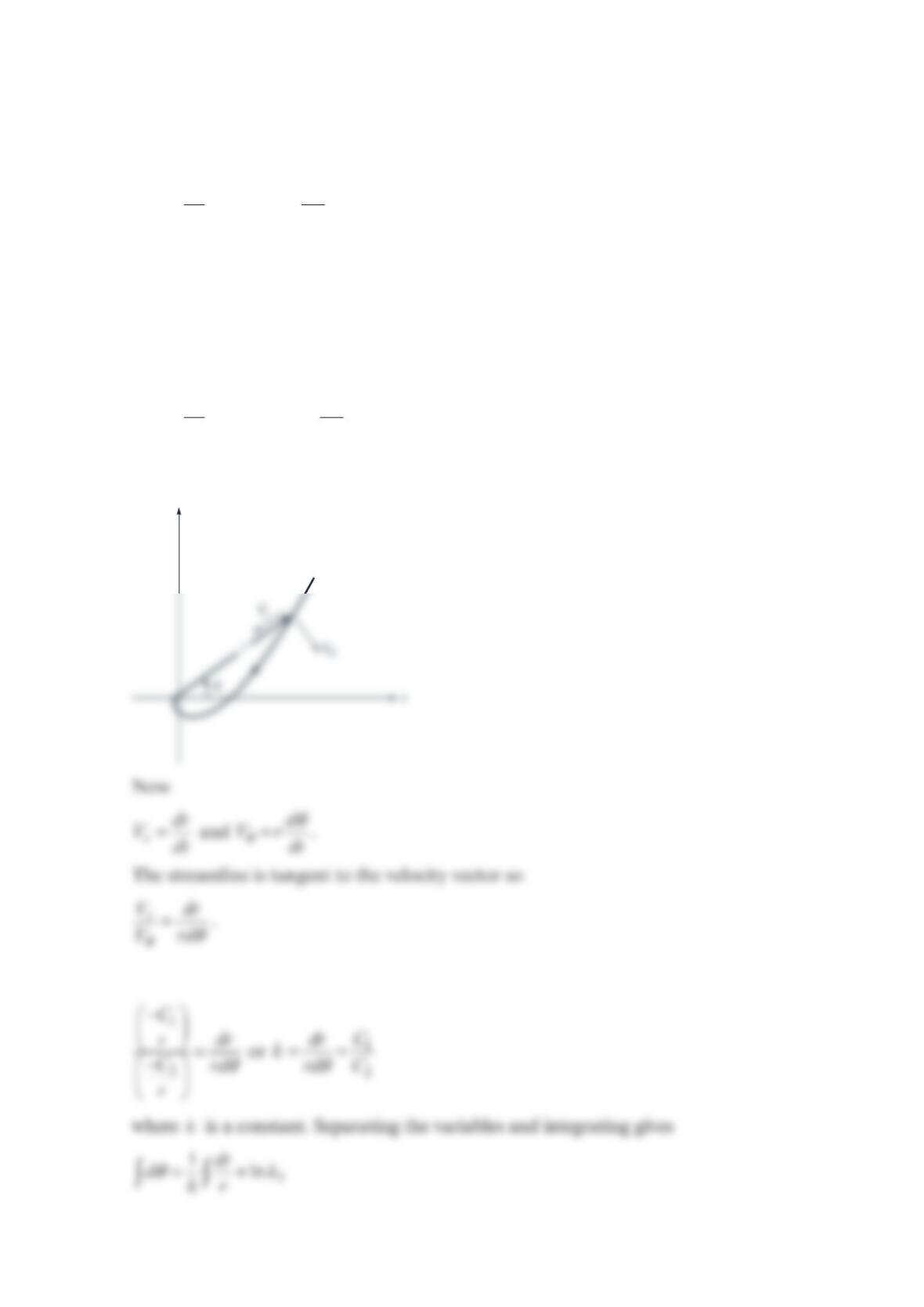
SOLUTION: First sketch the flow.
Substituting for r
V and
θ
V gives
y
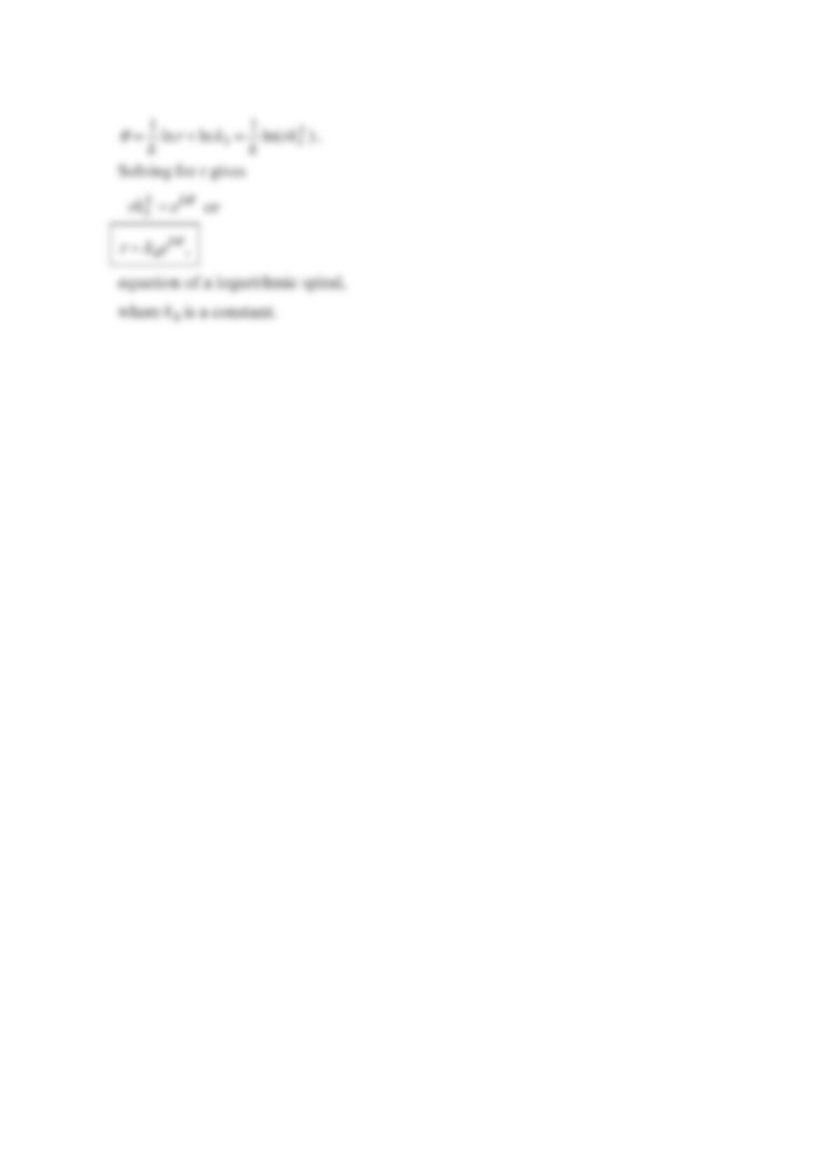
where 3
ln k is a constant. Integrating gives
Problem 4.18
THE WIDE WORLD OF FLUIDS
Follow those particles Superimpose two photographs of a bouncing ball taken a short time
apart and draw an arrow between the two images of the ball. This arrow represents an
approximation of the velocity (displacement/time) of the ball. The particle image
velocimeter (PIV) uses this technique to provide the instantaneous velocity field for a given
cross section of a flow. The flow being studied is seeded with numerous micronsized
particles that are small enough to follow the flow yet big enough to reflect enough light to
be captured by the camera. The flow is illuminated with a light sheet from a double-pulsed
laser. A digital camera captures both light pulses on the same image frame, allowing the
movement of the particles to be tracked. Using appropriate computer software to carry out
a pixel-by-pixel interrogation of the double image, it is possible to track the motion of the
particles and determine the two components of velocity in the given cross section of the
flow. Using two cameras in a stereoscopic arrangement, it is possible to determine all three
components of velocity.
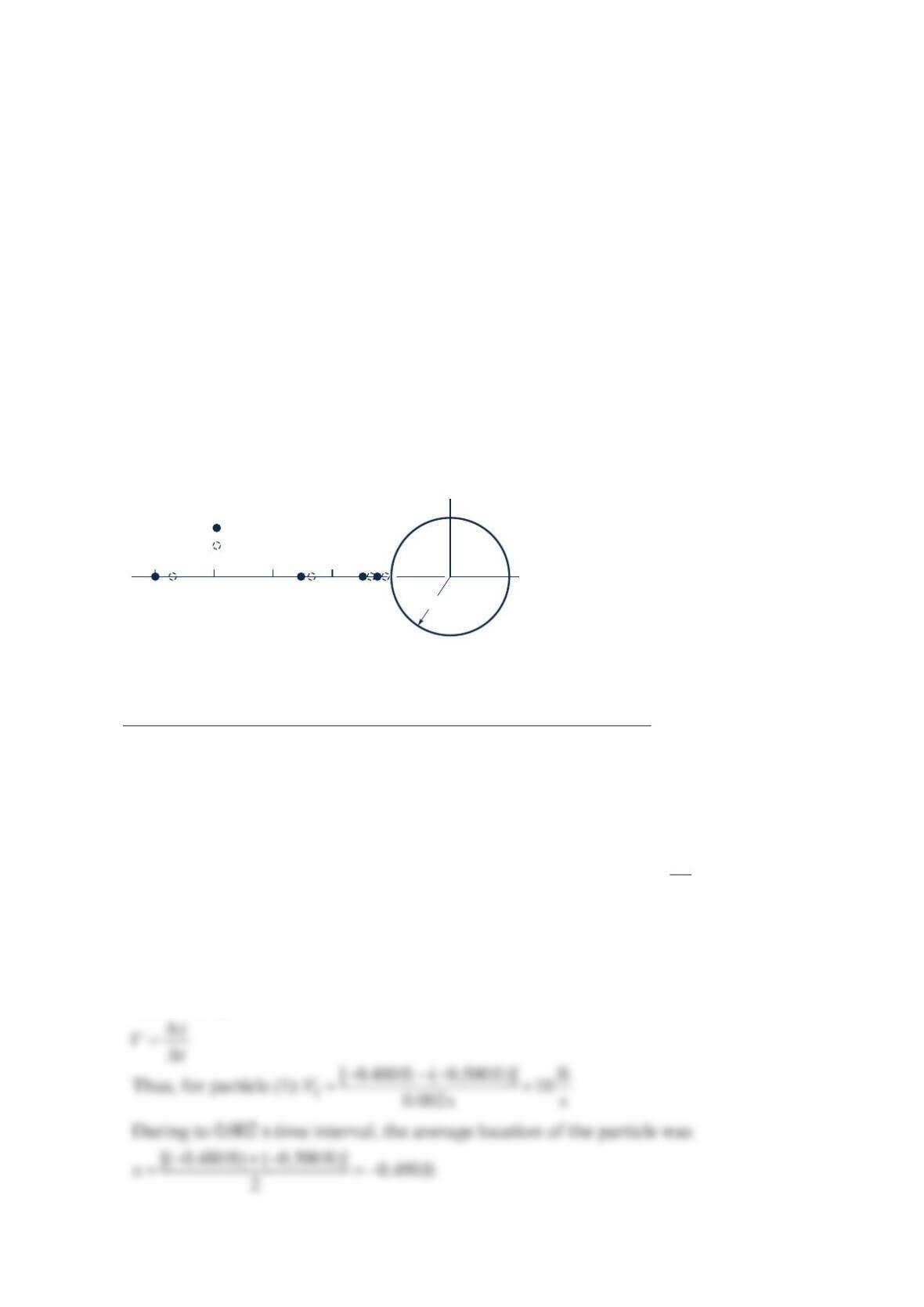
Two photographs of four particles in a flow past a sphere are superposed as shown in the
figure below.
The time interval between the photos is
Δ
=0.002 st. The locations of the particles, as
determined from the photos, are shown in the table.
Particle x at =0 s (ft)t x at =0.002 s (ft
)
t
1 0.500
−
0.480
−
2 0.250
−
0.232
−
3 0.140
−
0.128
−
4 0.120
−
0.112
−
(a) Determine the fluid velocity for these particles. (b) Plot a graph to compare the results
of part (a) with the theoretical velocity, which is given by
=+
3
03
1a
V
Vx, where a is the
sphere radius and 0
V
is the fluid speed far from the sphere.
Solution 4.18
The fluid velocity (which is assumed to be the same as the particle velocity) can be
estimated by
t
= 0
t
= 0.002 s
a
= 0.1 ft
y
, ft
x
, ft
–0.2–0.4
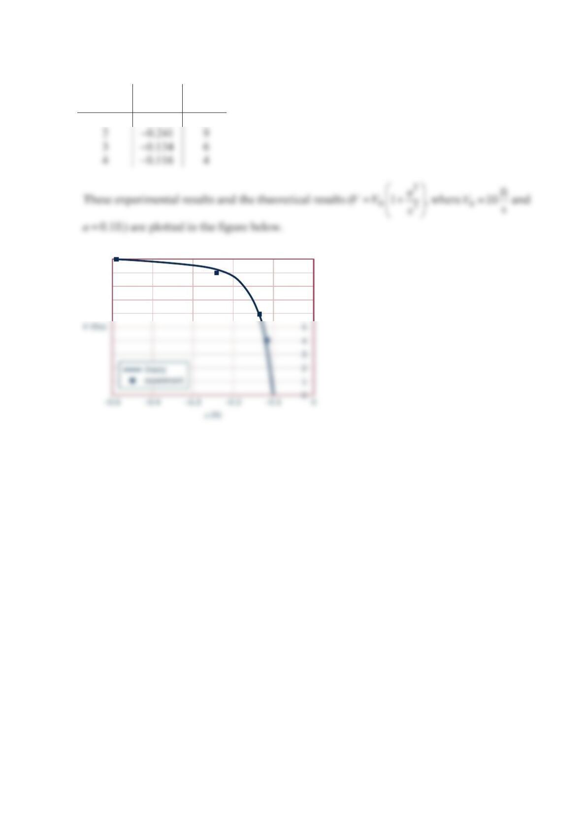
By similar calculations, the following experimental results were obtained:
Particle x (ft) V
(ft/s)
10.490
−
10
6
7
8
9
10
−
−
Problem 4.19
Air flows steadily through a circular, constant-diameter duct. The air is perfectly inviscid,
so the velocity profile is flat across each flow area. However, the air density decreases as the
air flows down the duct. Is this a one-, two-, or three-dimensional flow?
Solution 4.19
GIVEN: In viscid, steady, flow of air through a circular, constant diameter, duct with a flat
velocity profile at each flow area. Air density decreases as the air flows down the duct.
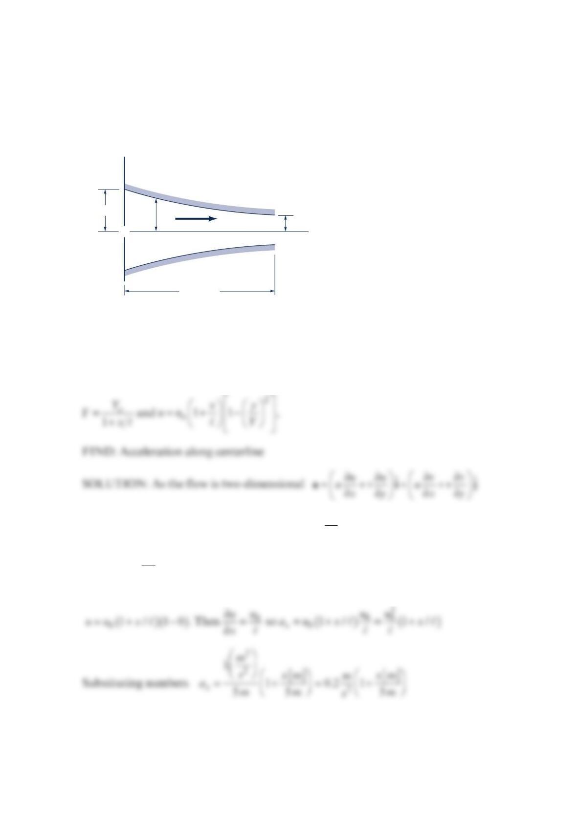
Problem 4.20
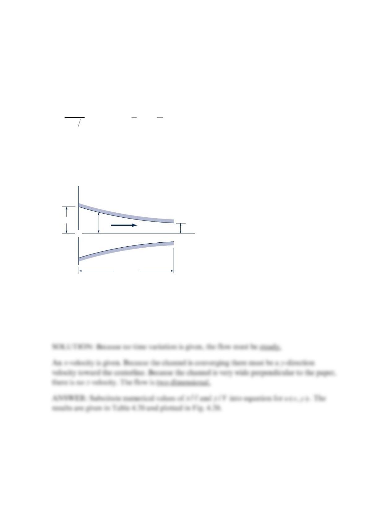
A constant-density fluid flows in the converging, two-dimensional channel as shown in the
figure below. The width perpendicular to the paper is quite large compared to the channel
height. The velocity in the z direction is zero. The channel half-height,
Y
, and the fluid x
velocity, u, are given by
=+
1
o
Y
Y
x and
=+ −
2
11 ,
o
xy
uu Y
where , , ,xyY
and
are in
m
eters,
u
is in
m
/s, =
o1.0 m/s,u and =
o1.0 m.Y (a) Is this
flow steady or unsteady? Is it one-dimensional, two-dimensional, or three-dimensional?
(b) Plot the velocity distribution
()
uy
at =
/
0,x0.5
,
and 1.0
.
Use /
y
Y values of 0,
±
0.2,
±
0.4,
±
0.6,
±
0.8, and
±
1.0
.
Solution 4.20
GIVEN: Channel with x-velocity distribution.
FIND: Is the flow steady or unsteady, one-, two-, or three-dimensional. Plot velocity
distribution.
x
y
+
ℓ = 5.0 m
Y
(
x
)
u
(
x, y
)
Y
0
= 1.0 m
Y
ℓ
= 0.5 m
/
y
Table 4.20. Tabulated values of the velocity (u,)xy as a function of the length ratio ,
the height ratio
/
yY
, and the height
y
for the two-dimensional channel.
Length Ratio x/ℓ Height Ratio y/Y Height y (m) Fluid Velocity u (m/s)
0.0 0.00 0.00 1.00
0.5 0.00 0.00 1.50
1.0 0.00 0.00 2.00
±0.20 ±0.10 1.92
Figure 4.20. Plot of the velocity (u,)xy as a function of the transverse coordinate
y
at
various axial locations.
y (m)
yy
1
1
1
Problem 4.22
Classify the following flows as one-, two-, or three-dimensional. Sketch a few streamlines
for each.
(a) Rainwater flow down a wide driveway
(b) Flow in a straight horizontal pipe
(c) Flow in a straight pipe inclined upward at a angle
(d) Flow in a long pipe that follows the ground in hilly country
(e) Flow over an airplane
(f) Wind blowing past a tall telephone
(g) Flow in the impeller of a centrifugal pump
Solution 4.22
(a) One-dimensional
Problem 4.23
The velocity components of u and v of a two-dimensional flow are given by
=+
22
bx
uaxxy
and =+
22
by
vayxy ,
where a and b are constants. Calculate the acceleration.
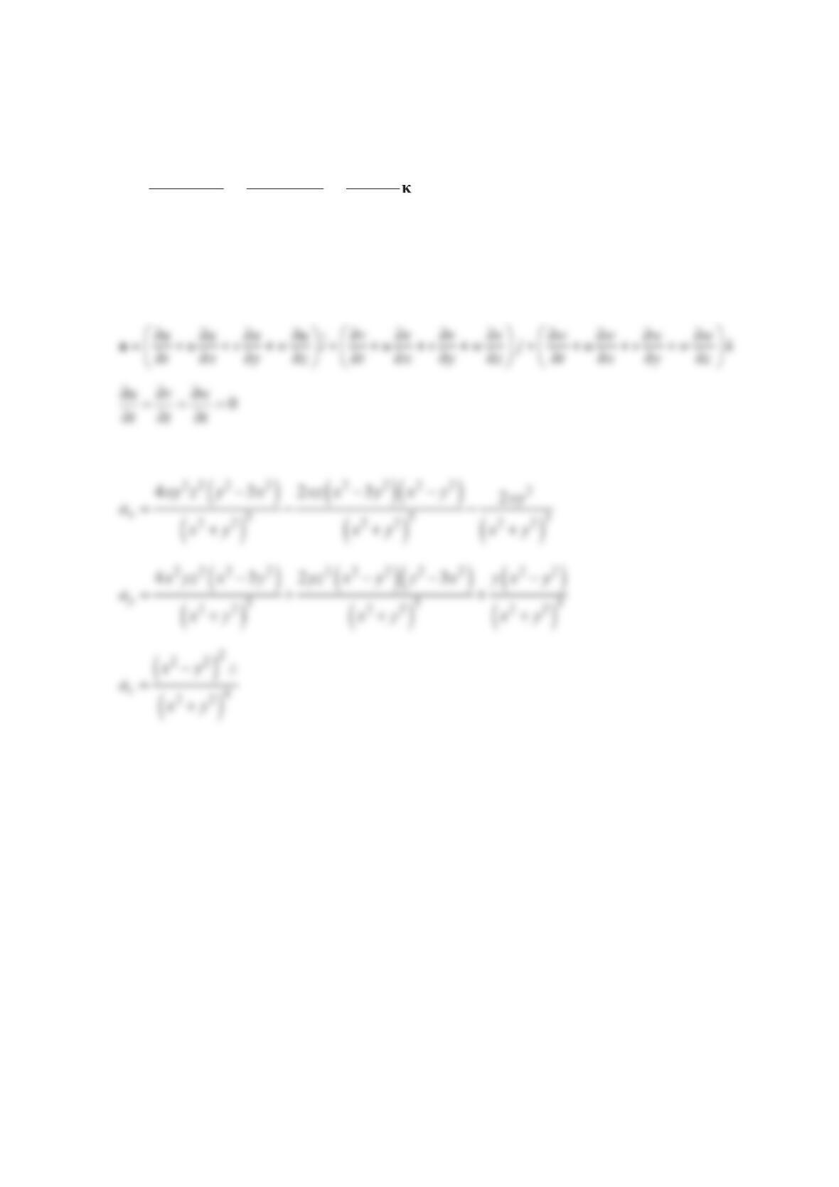
Solution 4.23
GIVEN: Velocity components
SOLUTION: Since the flow is spatially two-dimensional (,)xy and steady, the equations
are
Substituting into the equation for x
a gives
or
Substituting into the equation for y
a gives
or
=− +
22 22
3
y
bb
aya a
xy xy
Problem 4.24
Air is delivered through a constant-diameter duct by a fan. The air is inviscid, so the fluid
velocity profile is “flat” across each cross section. During the fan start-up, the following
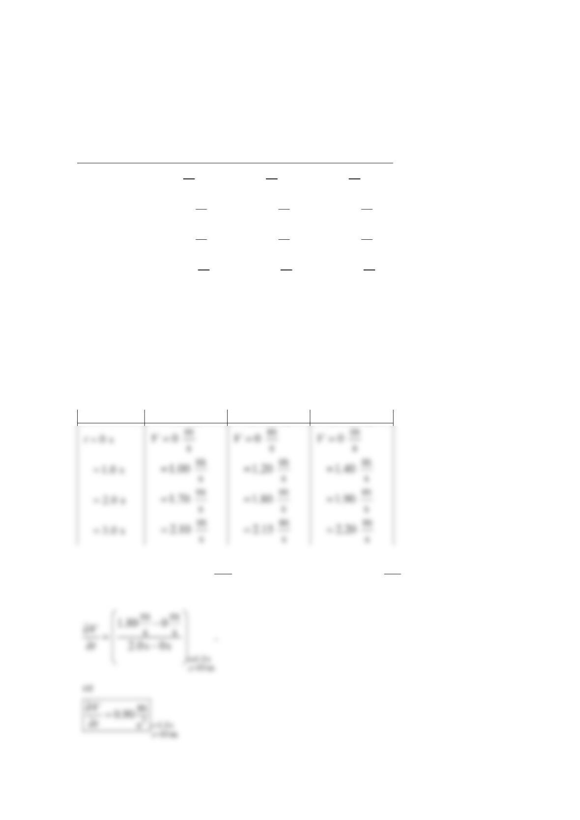
velocities were measured at the time t and axial positions x:
x = 0 x= 10 m x= 20 m
=0 st=m
0 s
V=m
0 s
V=m
0 s
V
=1.0 st=m
1.00 s
V=m
1.20 s
V=m
1.40 s
V
=2.0 st=m
1.70 s
V=m
1.80 s
V=m
1.90 s
V
=3.0 st=m
2.10 s
V=m
2.15 s
V=m
2.20 s
V
Calculate the local acceleration, the convective acceleration, and the total acceleration at
1.0 st= and 10 mx=. What is the local acceleration after the fan has reached a steady air
flowrate?
Solution 4.24
GIVEN: Air velocity in duct, axial position x at time t.
0x=10 mx=20 mx=
FIND: Local acceleration ∂
∂
V
t and convective acceleration ∂
∂
V
V
x at =1.0 st and =10
m
x.
SOLUTION: The local acceleration is
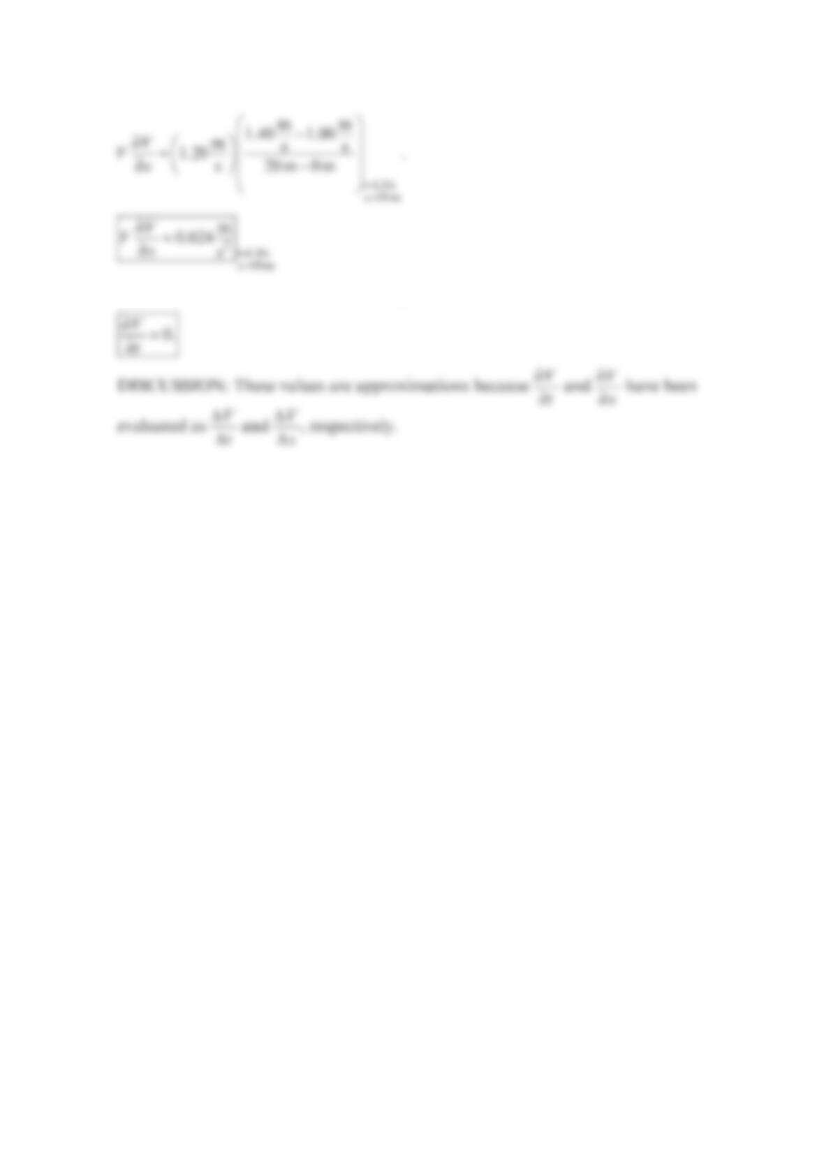
The convective acceleration is
When the air flowrate has become steady,
Problem 4.25
Water flows through a constant diameter pipe with a uniform velocity given by
=+
8m
5
st
V, where
t
is in seconds. Determine the acceleration at time =1, 2, and 10 st.
Solution 4.25
∂
=+⋅∇
∂t
V
aVV
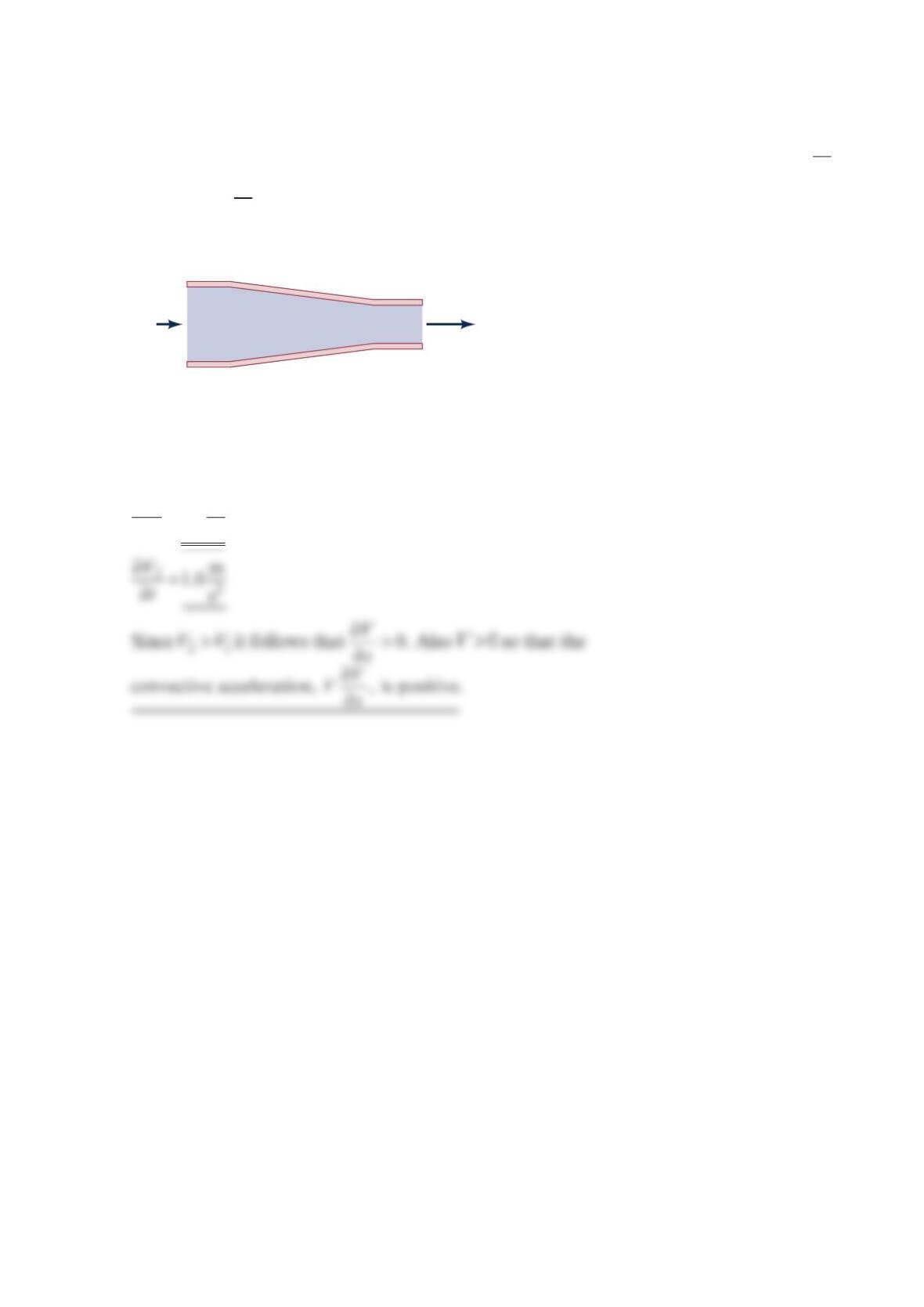
Problem 4.26
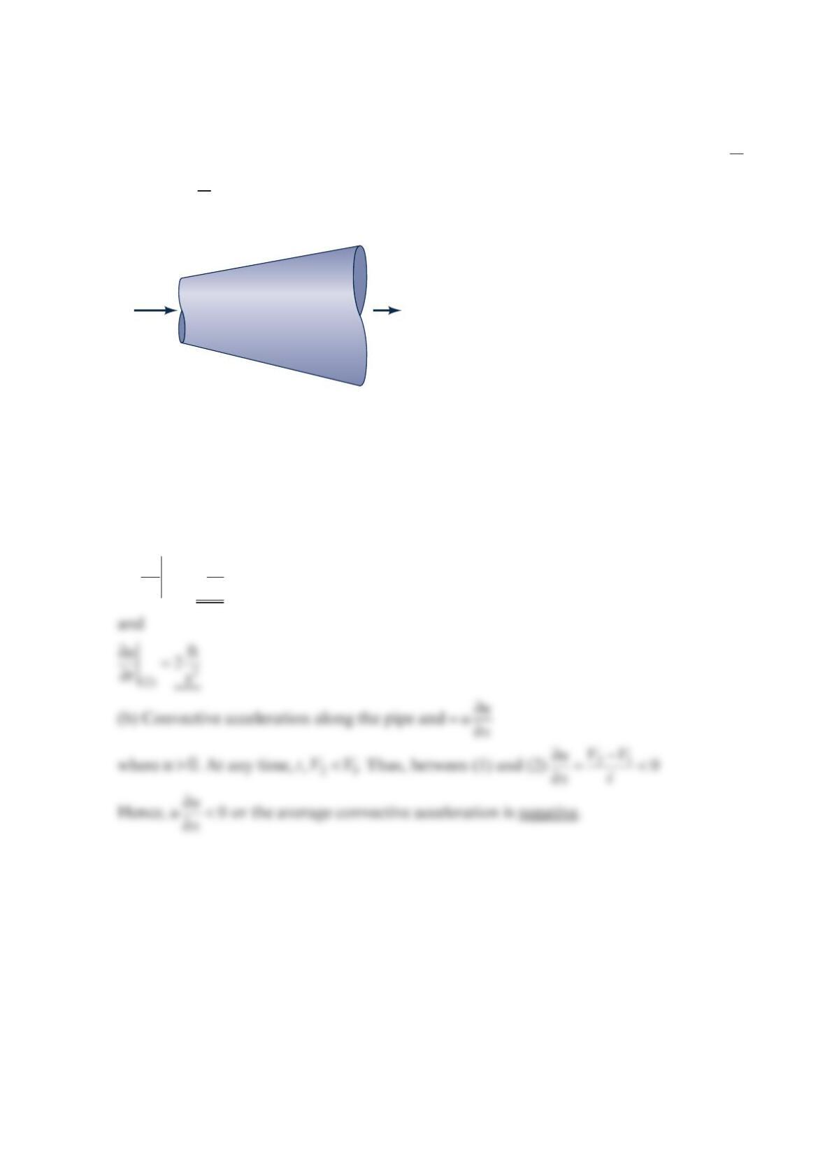
The velocity of air in the diverging pipe as shown in the figure below is given by =
1
ft
4s
V
t
and =
2
ft
2s
V
t, where
t
is in seconds.
(a) Determine the local acceleration at points (1) and (2). (b) Is the average convective
acceleration between these two points negative, zero, or positive? Explain.
Solution 4.26
(a) ∂=
∂2
(1)
ft
4s
u
t
V
1 = 4
t
ft/s
V
2 = 2
t
ft/s
(1)
(2)
Problem 4.27
A certain flow field has the velocity vector
()
()
()
−
−
=++
+
++
22
2222
22 22
2xyz
xyz y
xy
xy xy
Vij
. Find the acceleration vector for this flow.
Solution 4.27
=++uvwVijk
Using software to perform calculus and algebra results in:
Problem 4.28
Determine the –xcomponent of the acceleration, ,
x
a
along the centerline
()
=0y for the flow
of Problem 4.20. Can you determine the acceleration vector at a location not on the
centerline? Why or why not?
Solution 4.28
GIVEN: Flow from Problem 4.20
The flow is symmetric about the centerline so ∂
== =
∂0at
0
v
vy
y
Then ∂
==
∂and 0
xy
u
a
ua
x. Putting =
0
y
in the velocity distribution gives the centerline
velocity
x
y
+
ℓ = 5.0 m
Y
(
x
)
u
(
x, y
)
Y0
= 1.0 m
Yℓ
= 0.5 m
Problem 4.29
The velocity of the water in the pipe as shown in the figure below is given by =
1
m
0.50 s
V
t
and =
2
m
1.0 s
V
t, where
t
is in seconds. Determine the local acceleration at points (1) and
(2). Is the average convective acceleration between these two points negative, zero, or
positive? Explain.
Solution 4.29
∂=
∂
1
2
m
0.5 s
V
t
V
1 =
0.50
t
m/s
V
2 =
1.0
t
m/s
(1)
(2)
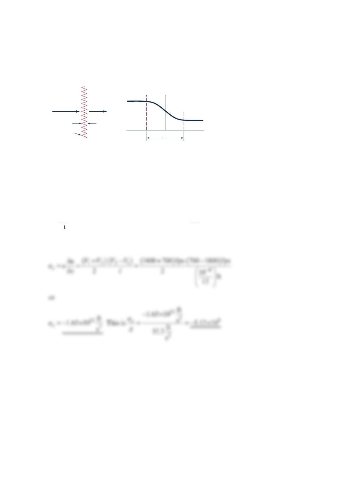
Problem 4.30
A shock wave is a very thin layer (thickness =
) in a highspeed (supersonic) gas flow across
which the flow properties (velocity, density, pressure, etc.) change from state (1) to state (2)
as shown in the figure below.
If =
11800 fpsV, =
2700 fpsV, and −
=4
10 in.
, estimate the average deceleration of the gas as
it flows across the shock wave. How manyg’s deceleration does this represent?
Solution 4.30
∂
=+⋅∇
∂
V
aVV
so that with =()
V
uxi
, ∂
==
∂
x
u
au
x
ai i
Without knowing the actual velocity distribution, =()uux
, the acceleration can be
approximated as
Shock wave
V2
V2
V1
V1
V
ℓ
ℓ
x