Section 3.3
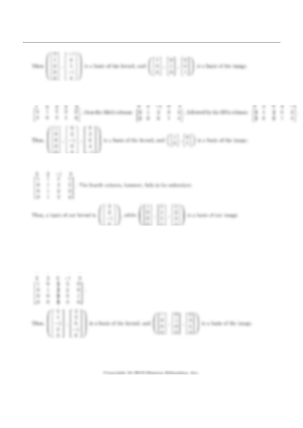
3.3.17 For this problem, we again successively use Kyle Numbers to find our kernel, investigating the columns from
left to right. We initially see that the first column is redunant:
3.3.18 The third column is redundant, as we find with
0
0
1
4
3.3.19 We see that the third column is redundant, and choose Kyle numbers as follows:
5 4 −1 0 0
1
0
0
0
0
1
0
0
5
4
0
0
3
2
0
0
0
0
1
0
, then we see that the fourth column is also redundant,
3.3.20 Although this matrix is not quite in rref, we can still quickly see that columns 2, 3, and 5 are the redundant
columns:
147
Chapter 3
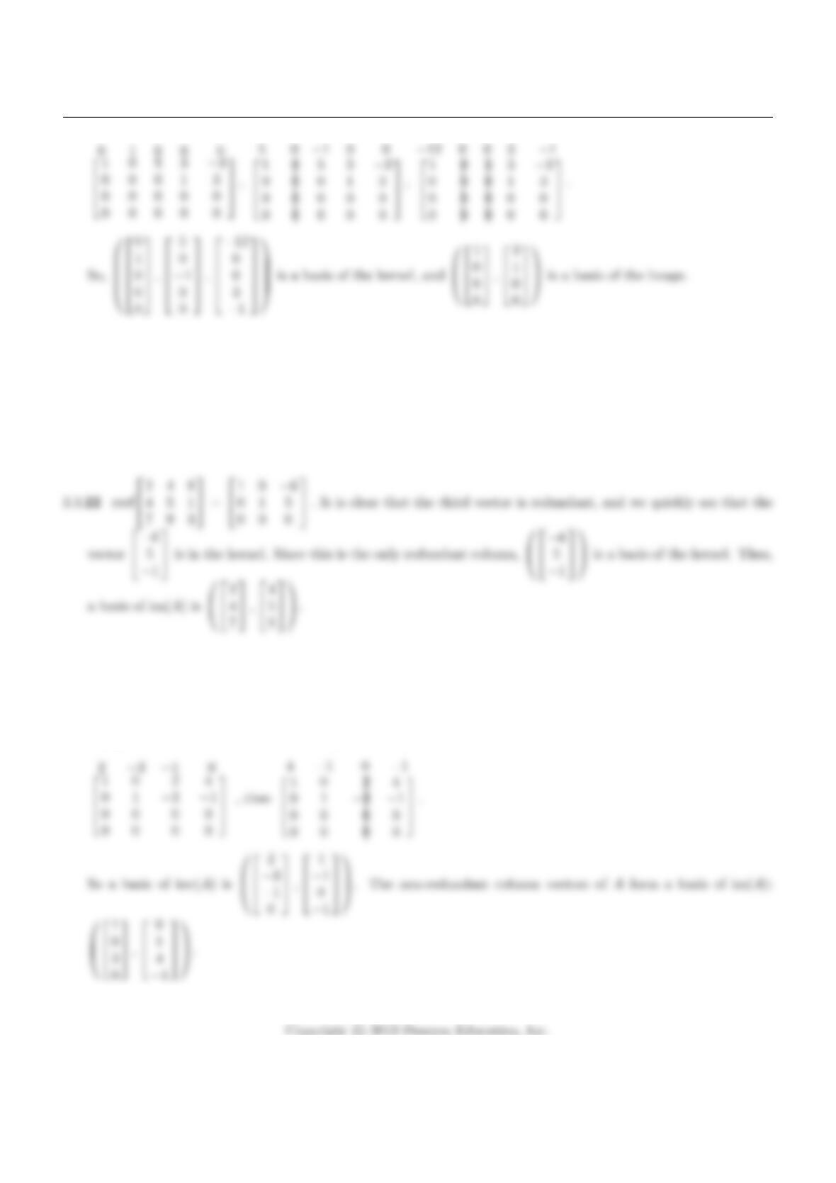
3.3.21 rref
1 3 9
4 5 8
7 6 3
=
1 0 −3
0 1 4
0 0 0
, which we can use to “spot” a vector in the kernel:
−3
4
−1
. Since the third
column is the only redundant one, this forms a basis of the kernel, and implies that the third column of Ais also
redundant. Thus, a basis of im(A) is
1
4
7
,
3
5
6
.
3.3.23 rref
1 0 2 4
0 1 −3−1
3 4 −6 8
0−1 3 1
=
1 0 2 4
0 1 −3−1
0 0 0 0
0 0 0 0
.
Using the method of Exercises 17 and 19, we find the kernel:
148
Section 3.3
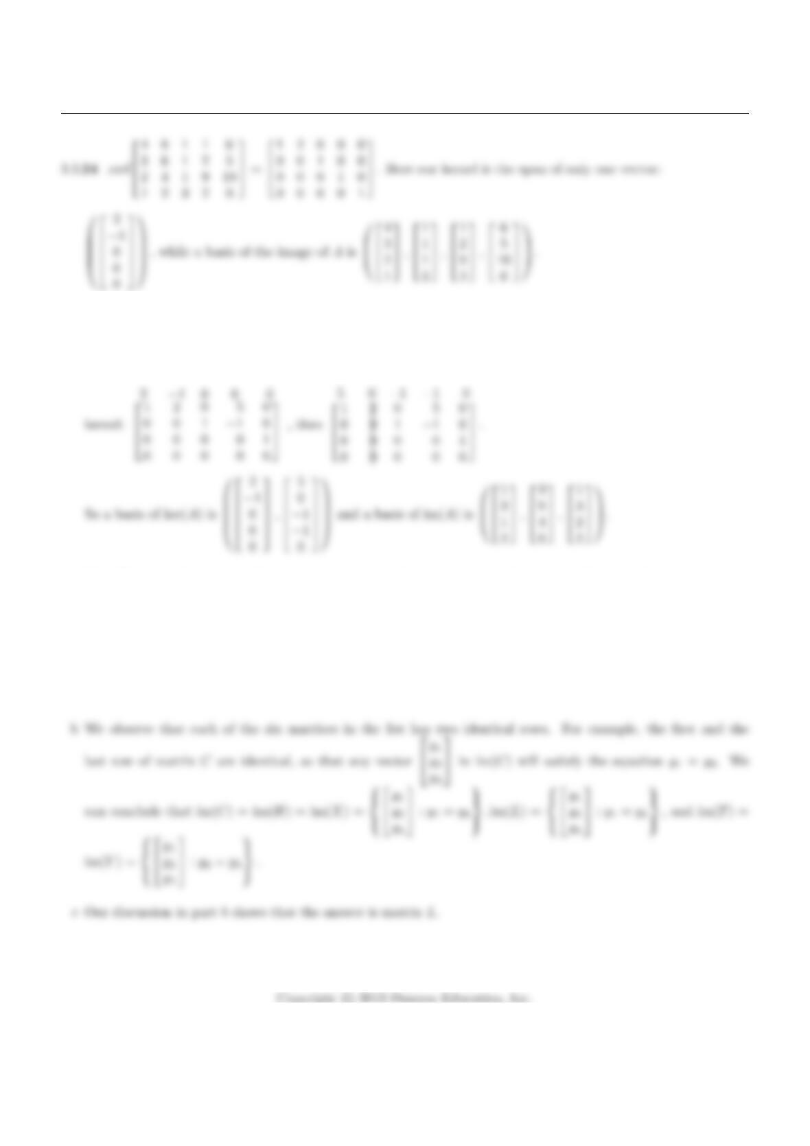
3.3.25 rref
1 2 3 2 1
3 6 9 6 3
1 2 4 1 2
2 4 9 1 2
=
1 2 0 5 0
0 0 1 −1 0
0 0 0 0 1
0 0 0 0 0
. We will emulate Exercise 23 to find the
3.3.26 a We notice that each of the six matrices has two identical columns. In matrices Cand L, the second column
is identical to the third, so that ker(C) = ker(L) = span
0
1
−1
.In matrices H, T, X and Y, the first column is
identical to the third, so that ker(H) = ker(T) = ker(X) = ker(Y) = span
1
0
−1
.Thus, only Lhas the same
kernel as C.
3.3.27 Form a 4 ×4 matrix Awith the given vectors as its columns. We find that rref(A) = I4, so that the vectors
149
Chapter 3
do indeed form a basis of R4, by Summary 3.3.10.
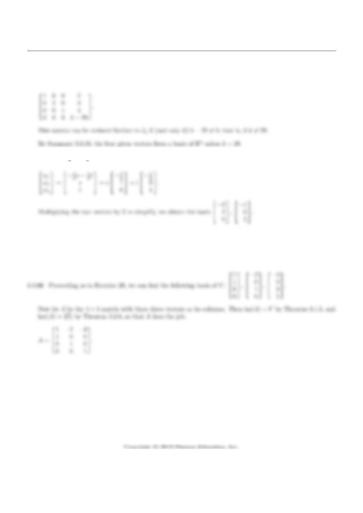
3.3.28 Form a 4 ×4 matrix Awith the given vectors as its columns. The matrix Areduces to
3.3.29 x1=−3
2x2−1
2x3; let x2=sand x3=t. Then the solutions are of the form
3.3.30 Proceeding as in Exercise 29, we find the basis
1
2
0
0
,
−1
0
1
0
,
−2
0
0
1
.
3.3.32 We need to find all vectors ~x in R4such that
x1
x2
x3
x4
·
1
0
−1
1
= 0 and
x1
x2
x3
x4
·
0
1
2
3
= 0.
This amounts to solving the system x1−x3+x4= 0
x2+ 2x3+ 3x4= 0 , which in turn amounts to finding the
kernel of 1 0 −1 1
0 1 2 3 .
150
Section 3.3
3.3.33 We can write V= ker(A), where Ais the 1 ×nmatrix A= [c1c2··· cn].
3.3.34 We can write V= ker(A), where Ais the n×mmatrix with entries aij . Note that rank(A)≤n. Therefore,
dim(V) = dim(ker(A)) = m−rank(A)≥m−n, by Theorem 3.3.7.
3.3.37 Since dim(ker(A)) = 5 −rank(A), any 4 ×5 matrix with rank 2 will do; for example,
A=
10000
01000
00000
00000
.
3.3.39 Note that ker(C)6={~
0}, by Theorem 3.1.7a, and ker(C)⊆ker(A). Therefore, ker(A)6={~
0}, so that Ais not
invertible.
3.3.41 The kernel of a 4 ×6 matrix is at least two-dimensional. Since every one-dimensional subspace of this kernel
defines a conic through the four given points, there will be infinitely many such conics.
3.3.42 The kernel of a 5 ×6 matrix is at least one-dimensional, so that there is at least one conic passing through
3.3.43 Here, “anything can happen”:
Chapter 3
1. If ker A=n~
0o, then there is no solution, as in Exercise 1.2.61.
3.3.44 The conic runs through the point (0,0) if c1= 0.
Now the conic runs through (1,0) and (2,0) if c2+c4+c7= 0 and 2c2+ 4c4+ 8c7= 0. We find that c2= 2c7
3.3.45 The conic runs through the point (0,0) if c1= 0.
Now the conic runs through (1,0), (2,0), and (3,0) if c2+c4+c7= 0, 2c2+4c4+8c7= 0, and 3c2+ 9c4+ 27c7= 0.
Solving this system, we find that c2=c4=c7= 0.
Likewise, the conic runs through (0,1) (0,2), and (0,3) if c3=c6=c10 = 0.
-1
-1
3
2
4
421
x
y
3
1
-1
-1
3
2
4
421
x
y
3
1
3.3.47 To run through the points (0,0) ,(1,0) ,(2,0), and (3,0), the cubic must satisfy the equations c1= 0, c1+
c2+c4+c7= 0, c1+ 2c2+ 4c4+ 8c7= 0,and c1+ 3c2+ 9c4+ 27c7= 0. This means that c1=c2=c4=c7= 0.
Likewise, the cubic runs through the points (0,0) ,(0,1) ,(0,2) and (0,3) if (and only if) c1=c3=c6=c10 = 0.
Section 3.3
3
4
y
3.3.48 Here we add the point (4,0) to the list of points in Exercise 46. In Exercise 46 we found the family of cubics
xy (ax +by −a−b) = 0, where a6= 0 or b6= 0. Since all these cubics run through the point (4,0), we find the
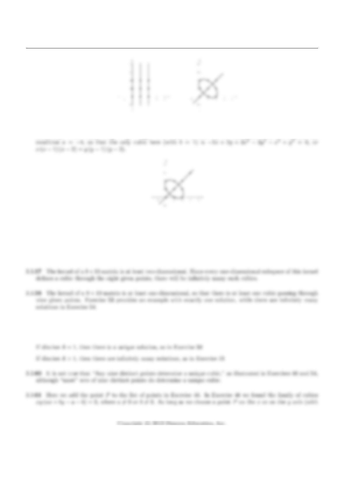
same solutions here: xy (ax +by −a−b) = 0, where a6= 0 or b6= 0. Two sample solutions are shown in the
accompanying figures.
3.3.49 Here we add the point (2,1) to the list of points in Exercise 47. In Exercise 47 we found the cubic xy (y−x) =
0. Since this cubic fails to run through the point (2,1), there are no solutions here.
3
4
y
3.3.50 Here we add the point (3,3) to the list of points in Exercise 47. In Exercise 47 we found the cubic xy (y−x) =
0. Since this cubic runs though the point (3,3), we get the same solution here, xy (y−x) = 0.
4
y
3.3.51 Here we add the point (0,4) to the list of points in Exercise 48. In Exercise 48 we found the family of cubics
xy (ax +by −a−b) = 0, where a6= 0 or b6= 0. Since all these cubics run through the point (0,4), we find the
153
Chapter 3
3.3.52 To run through the points (0,0) ,(1,0) ,and (2,0), the cubic must satisfy the equations c1= 0, c1+c2+c4+
c7= 0,and c1+ 2c2+ 4c4+ 8c7= 0. This means that c1= 0, c2= 2c7and c4=−3c7. Likewise, the cubic runs
through the points (0,0) ,(0,1) ,and (0,2) if (and only if) c1= 0, c3= 2c10 and c6=−3c10. Therefore, to run
through the points (0,0),(1,0),(2,0),(0,1),(0,2) the cubic must be of the form c5xy +c7x3−3x2+ 2x+
3.3.53 Here we add the point (3,2) to the list of points in Exercise 52. In Exercise 52 we found the family of cubics
3.3.54 Here we add the point (2,2) to the list of points in Exercise 52. In Exercise 52 we found the family of cubics
ax3−3x2+ 2x+by3−3y2+ 2y= 0 , where a6= 0 or b6= 0. Since all these cubics run through the point
(2,2), we find the same solutions here: ax3−3x2+ 2x+by3−3y2+ 2y= 0 , where a6= 0 or b6= 0. Two
sample solutions are shown in the accompanying figures.
154
Section 3.3
3.3.55 Here we add the point (3,3) to the list of points in Exercise 54 In Exercise 54 we found the family of
cubics ax3−3x2+ 2x+by3−3y2+ 2y= 0 , where a6= 0 or b6= 0. The point (3,3) now imposes the
3.3.56 Substituting a point (x, y) = (xi, yi) into the equation c1+c2x+… +c9xy2+c10y3= 0 produces a linear
equation in the ten unknows c1, …, c10. Fitting a cubic through mpoints Pi(xi, yi), for i= 1, …, m, amounts to
solving a system of mhomogenous linear equations in ten unknowns. This system can be written in matrix form
as A~x =~
0, where Ais an m×10 matrix. The ith row of Ais 1xiyix2
ixiyiy2
ix3
ix2
iyixiy2
iy3
i
.
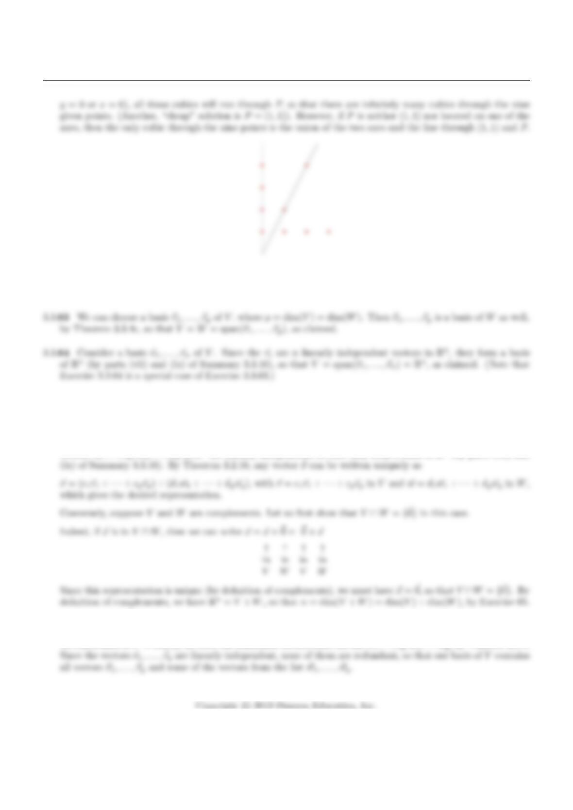
3.3.57 Here, “anything can happen”:
If ker A=n~
0o, then there is no solution, as in Exercise 49
155
Chapter 3
3.3.62 We can choose a basis ~v1, . . . , ~vpin V, where p= dim(V). Then ~v1, . . . , ~vpare linearly independent vectors
in W, so that dim(V) = p≤dim(W), by Theorem 3.3.4a, as claimed.
3.3.65 dim(V+W) = dim(V) + dim(W), by Exercise 3.2.51b.
3.3.66 Suppose that V∩W={~
0}and dim(V) + dim(W) = n.
Choose a basis ~v1, . . . , ~vpof Vand a basis ~w1, . . . , ~wqin W; note that p+q=n. By Exercise 3.2.51b, the n
vectors ~v1, . . . , ~vp, ~w1, . . . , ~wqin Rnare linearly independent, so that they form a basis of Rn(by parts (vii) and
3.3.67 Note that im(A) = span(~v1, . . . , ~vp, ~w1, . . . , ~wq) = V, since the ~wjalone span V.
To find a basis of V= im(A), we omit the redundant vectors from the list ~v1, . . . , ~vp, ~w1, . . . ~wq, by Theorem 3.2.4.
156
Section 3.3
3.3.68 Use Exercise 67 with ~v1=
1
2
3
4
,~v2=
1
4
6
8
, and ~wi=~eifor i= 1,2,3,4.
3.3.69 Using the terminology suggested in the hint, we need to show that
~u1, . . . , ~um, ~v1, . . . , ~vp, ~w1, . . . , ~wq
is a basis of V+W. Then dim(V+W) + dim(V∩W) = (m+p+q) + m= (m+p) + (m+q) = dim(V) + dim(W),
3.3.70 By Exercise 3.3.69, dim(V∩W) = dim(V) + dim(W)−dim(V+W) = 13 −dim(V+W).
The dimension of V+Wis at least 7 (since W⊆V+W) and at most 10 (since V+W⊆R10); therefore the
dimension of V∩Wis at least 3 and at most 6.
3.3.74 rref(A) =
1 0 −1−2
0 1 2 3
0 0 0 0
0 0 0 0
157
Chapter 3
By Exercises 3.3.72 and 3.3.73a, [1 0 −1−2],[0 1 2 3] is a basis of the row space of A.
3.3.76 We can use the approach outlined in Exercise 3.3.75, with ~v =1
0, say.
3.3.77 If rank(A) = n, then the nnon-redundant columns of Aform a basis of im(A) = Rn, so that the matrix
formed by the non-redundant columns is invertible (by Summary 3.3.10).
Conversely, if Ahas an invertible n×nsubmatrix B, then the columns of Bform a basis of Rn(again by
Summary 3.3.10), so that im(A) = Rnand therefore rank(A) = dim(im(A)) = n.
3.3.79 As in Exercise 78, let mbe the smallest positive integer such that Am= 0. In Exercise 78 we construct m
linearly independent vectors ~v, A~v, . . . , Am−1~v in Rn; now m≤nby Theorem 3.2.8.
Therefore An=AmAn−m= 0An−m= 0, as claimed.
3.3.82 im(A) is the plane onto which we project, so that rank(A) = dim(im(A)) = 2.
3.3.83 a Note that rank(B)≤2, so that dim(ker(B)) = 5 −rank(B)≥3 and dim(ker(AB)) ≥3 since ker(B)⊆
ker(AB). Since ker(AB) is an subspace of R5, dim(ker(AB)) could be 3,4, or 5. It is easy to give an example
158
Section 3.3
3.3.84 Write A= [~v1. . . ~vm] and B= [ ~w1. . . ~wm], so that A+B= [~v1+~w1···~vm+~wm]. Any linear combination
of the columns of A+B, ~y =c1(~v1+~w1) + ···+cm(~vm+~wm), can be written as
3.3.85 a By Exercise 3.1.39b, im(AB)⊆im(A), and therefore rank(AB)≤rank(A).
b Write B= [~v1··· ~vm] and AB = [A~v1··· A~vm]. If r= rank(B), then the rnon-redundant columns of Bwill
span im(B), and the corresponding rcolumns of AB will span im(AB), by linearity of A. By Theorem 3.3.4b,
rank(AB) = dim(im(AB)) ≤r= rank(B).
Summary: rank(AB)≤rank(A), and rank(AB)≤rank(B).
3.3.88 We will freely use the terminology introduced in the hint. First we need to show that at least one of the
column vectors ~akand ~
bkfails to contain a leading 1. If rank[~a1··· ~ak−1] = rank h~
b1··· ~
bk−1i=r, and if ~ak
159
Chapter 3
3.3.89 Exercise 88 shows that if two matrices Aand Bof the same size are both in rref and have the same kernel,
then A=B. Apply this fact to Aand B= rref(M).
3.3.90 We have T(~x) = ~v ×~x =~
0 if (and only if) the vector ~x is parallel to ~v (by Definition A.9). This means that
ker(T) = span(~v), a line.
Section 3.4
3.4.12
3= 2 1
0+ 3 0
1, so [~x]B=2
3.
3.4.223
29 =1
246
58 + 0 61
67 , so [~x]B=1
2
0.
This may not be as obvious as Exercises 1 and 3, but we can find our coefficients simply by reducing the matrix
2 5
5 12
.
.
.7
16 .
160
Section 3.4
3.4.8−4
4= 11 1
2−35
6, so [~x]B=11
−3.
We arrive at this solution by reducing the matrix 1 5
2 6
.
.
.−4
4.
3.4.9We can solve this by inspection: Note that our first coefficient must be 3 because of the first terms of the
vectors. Also, the second coefficient must be 2 due to the last terms.
V.
3.4.10 Proceeding as in Example 1, we find [~x]B=−3
5.
3.4.11 Proceeding as in Example 1, we find [~x]B=1
2
1
2.
3.4.14 We reduce
1 1 1
1 2 3
1 3 6
.
.
.
7
1
3
to
1 0 0
0 1 0
0 0 1
.
.
.
21
−22
8
,
Chapter 3
3.4.16 We proceed by inspection here, noting that we need c1= 3,then see that c2must be 4. Finally, c3must be
6.
3.4.18 Here, ~x is not in V, as we find an inconsistency while attempting to solve the system.
3.4.19 aS=1 1
1−1, and we find the inverse S−1to be equal to 1
21 1
1−1.
cB= [[T(~v1)]B[T(~v2)]B] = 0 1
1 0 1
1B0 1
1 0 1
−1B=1
1B−1
1B=1 0
0−1.
b Our commutative diagram:
162