PROBLEM 3.57
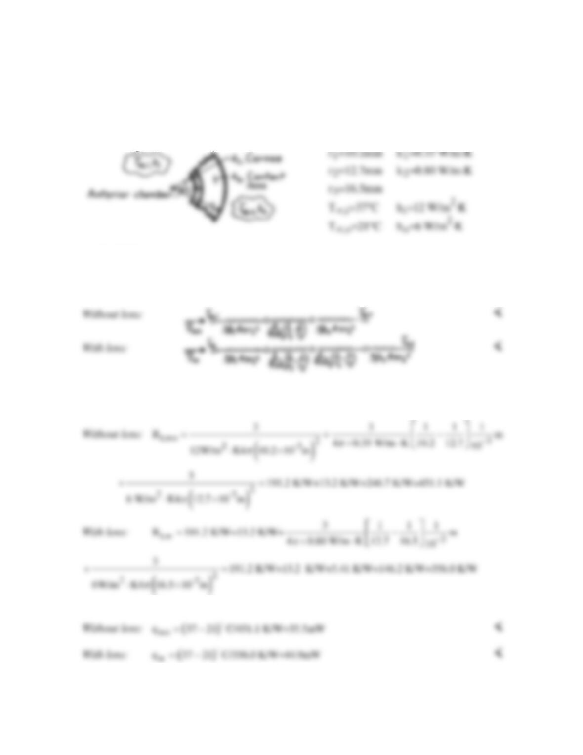
KNOWN: Representation of the eye with a contact lens as a composite spherical system subjected to
convection processes at the boundaries.
FIND: (a) Thermal circuits with and without contact lens in place, (b) Heat loss from anterior
chamber for both cases, and (c) Implications of the heat loss calculations.
SCHEMATIC:
ASSUMPTIONS: (1) Steady-state conditions, (2) Eye is represented as 1/3 sphere, (3) Convection
coefficient, ho, unchanged with or without lens present, (4) Negligible contact resistance.
ANALYSIS: (a) Using Eqs. 3.9 and 3.41 to express the resistance terms, the thermal circuits are:
(b) The heat losses for both cases can be determined as q = (T∞,i – T∞,o)/Rt, where Rt is the
thermal resistance from the above circuits.
Hence the heat loss rates from the anterior chamber are
(c) The heat loss from the anterior chamber increases by approximately 20% when the contact
lens is in place, implying that the outer radius, r3, is less than the critical radius.
PROBLEM 3.58
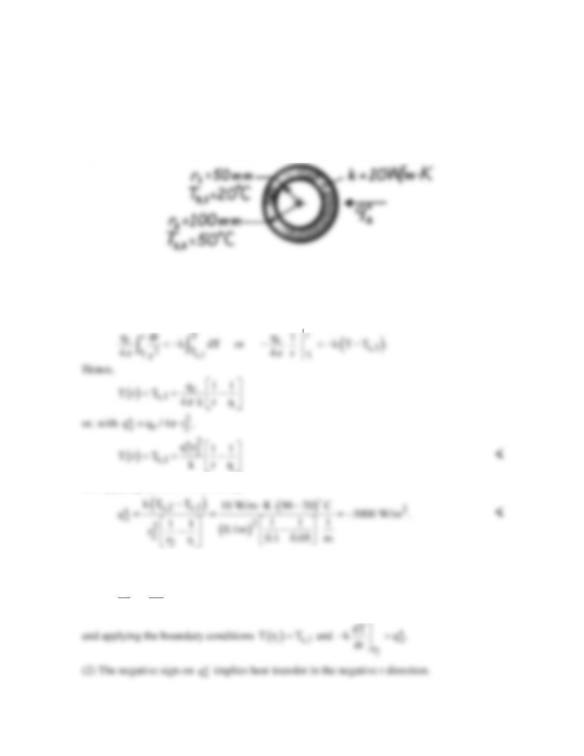
KNOWN: Thermal conductivity and inner and outer radii of a hollow sphere subjected to a
uniform heat flux at its outer surface and maintained at a uniform temperature on the inner
surface.
FIND: (a) Expression for radial temperature distribution, (b) Heat flux required to maintain
prescribed surface temperatures.
SCHEMATIC:
ASSUMPTIONS: (1) Steady-state conditions, (2) One-dimensional radial conduction, (3)
No generation, (4) Constant properties.
ANALYSIS: (a) For the assumptions, the temperature distribution may be obtained by
integrating Fourier’s law, Eq. 3.38. That is,
(b) Applying the above result at r2,
COMMENTS: (1) The desired temperature distribution could also be obtained by solving
the appropriate form of the heat equation,
2
d dT
r0
dr dr
=
PROBLEM 3.59
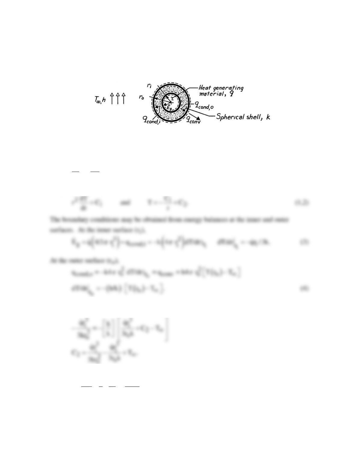
KNOWN: Volumetric heat generation occurring within the cavity of a spherical shell of
prescribed dimensions. Convection conditions at outer surface.
FIND: Expression for steady–state temperature distribution in shell.
SCHEMATIC:
ASSUMPTIONS: (1) One-dimensional radial conduction, (2) Steady-state conditions, (3)
Constant properties, (4) Uniform generation within the shell cavity, (5) Negligible radiation.
ANALYSIS: For the prescribed conditions, the appropriate form of the heat equation is
2
d dT
r0
dr dr
=
Integrate twice to obtain,
From Eqs. (1) and (3),
3
1i
C qr / 3k.= −
From Eqs. (1), (2) and (4)
Hence, the temperature distribution is
33
ii
2
oo
qr qr
11
T= T .
3k r r 3hr ∞
−+ +
<
COMMENTS: Note that
.E q q q
g cond,i cond,o conv
= = =
PROBLEM 3.60
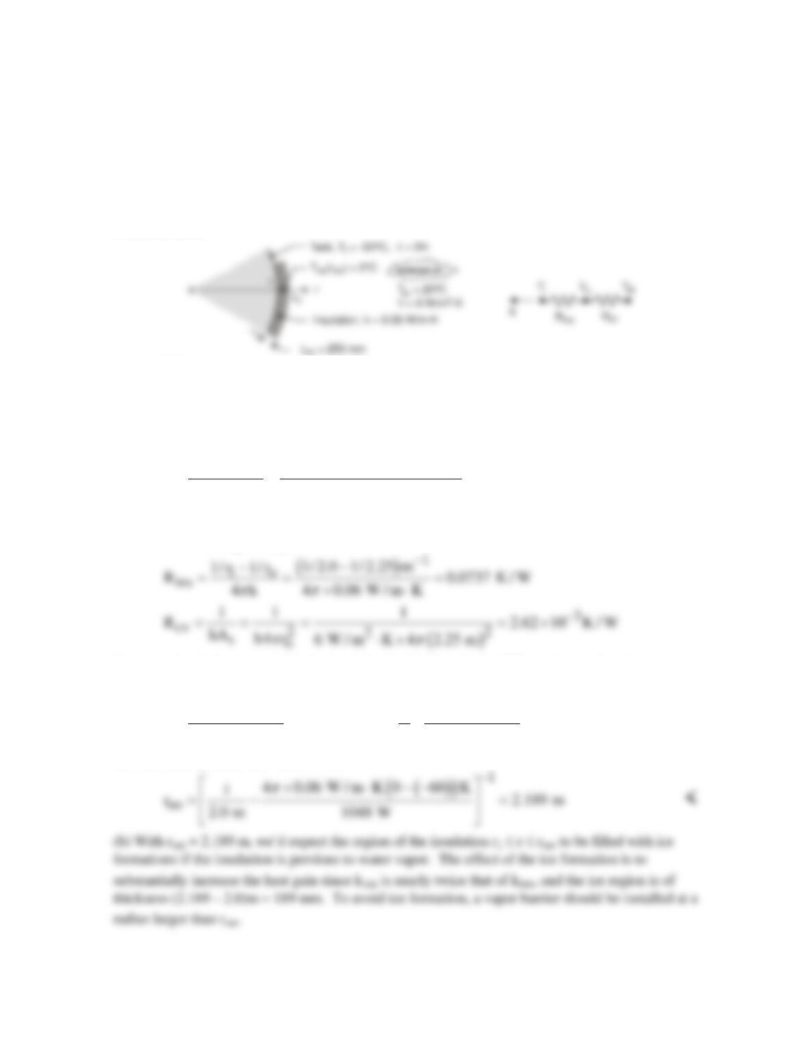
KNOWN: Spherical tank of 4-m diameter containing LP gas at -60°C with 250 mm thickness of
insulation having thermal conductivity of 0.06 W/m⋅K. Ambient air temperature and convection
coefficient on the outer surface are 20°C and 6 W/m2⋅K, respectively.
FIND: (a) Determine the radial position in the insulation at which the temperature is 0°C and (b) If
the insulation is pervious to moisture, what conclusions can be reached about ice formation? What
effect will ice formation have on the heat gain? How can this situation be avoided?
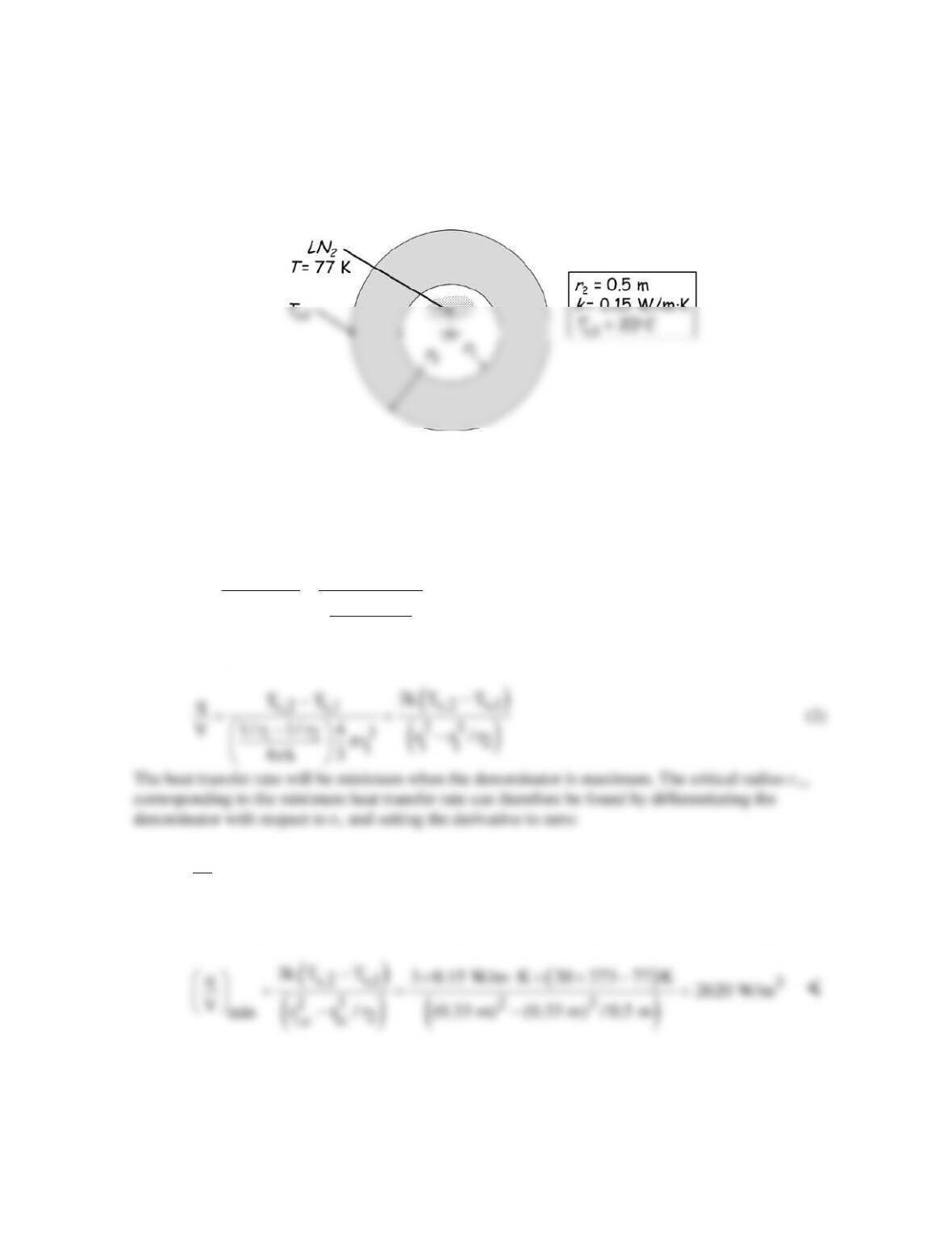
SCHEMATIC:
ASSUMPTIONS: (1) Steady-state conditions, (2) One-dimensional, radial (spherical) conduction
through the insulation, and (3) Negligible radiation exchange between the insulation outer surface and
the ambient surroundings, (4) Inner surface of insulation at Tt.
ANALYSIS: (a) The heat transfer situation can be represented by the thermal circuit shown above.
The heat gain to the tank is
( )
()
t
3
ins cv
20 60 K
TT
q 1048 W
RR 0.0737 2.62 10 K / W
∞−
−−
−
= = =
++×
where the thermal resistances for the insulation (see Table 3.3) and the convection process on the
outer surface are, respectively,
To determine the location within the insulation where Too (roo) = 0°C, use the conduction rate
equation, Eq. 3.41,
( )
( )
( )
1
oo t oo t
oo
i oo i
4kT T 4kT T
1
qr
1/r 1/ r r q
ππ
−
−−
= = −
−
and substituting numerical values, find
PROBLEM 3.61
KNOWN: Spherical tank of liquid nitrogen insulated with layer of known thermal conductivity and
outer radius. Inner and outer temperatures.
FIND: Radius of tank that minimizes heat transfer rate and value of minimum heat transfer rate per
unit nitrogen volume.
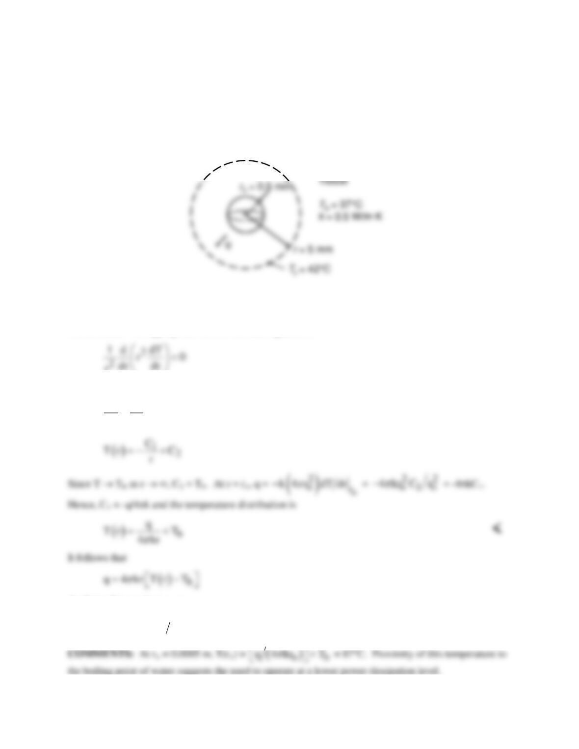
SCHEMATIC:
ASSUMPTIONS: (1) Steady-state conditions, (2) One-dimensional, radial (spherical) conduction
through the insulation, and (3) Inner surface of insulation at T = 77 K.
PROPERTIES: Given, k = 0.15 W/m⋅K.
ANALYSIS: The heat gain to the tank is
s,2 s,1 s,2 s,1
12
ins
TT TT
q1/r 1/ r
R
4k
π
−−
= = −
(1)
The heat rate per unit volume of nitrogen is
()
23 2
2 1 2 1,c 2
11 1
dr r / r 2r 3r / r 0, r 2r / 3 2 0.5 m / 3 0.33 m
dr −=−= ==× =
<
The corresponding minimum heat transfer rate per volume of nitrogen can be found from Eq. (2):
COMMENTS: The existence of a minimum heat transfer rate per nitrogen volume occurs because as
r1 is reduced (insulation thickness is increased), the heat transfer rate decreases, but so does the
nitrogen volume.
PROBLEM 3.62
KNOWN: Critical and normal tissue temperatures. Radius of spherical heat source and radius of tissue
to be maintained above the critical temperature. Tissue thermal conductivity.
FIND: General expression for radial temperature distribution in tissue. Heat rate required to maintain
prescribed thermal conditions.
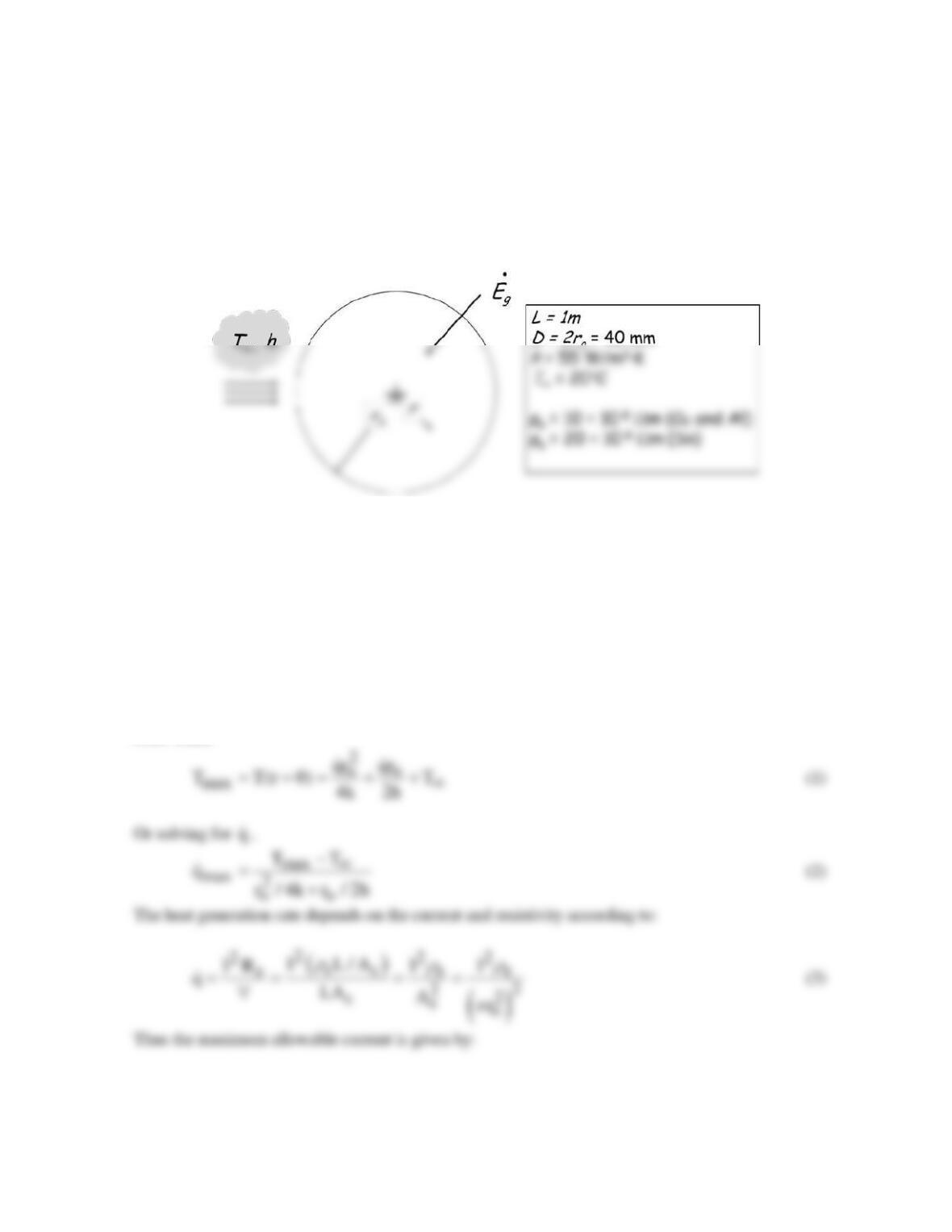
SCHEMATIC:
ASSUMPTIONS: (1) One-dimensional, steady-state conduction, (2) Constant k, (3) Negligible contact
resistance.
ANALYSIS: The appropriate form of the heat equation is
r
Integrating twice,
1
2
dT C
dr r
=
Applying this result at r = rc,
( )( )
( )
q 4 0.5 W m K 0.005 m 42 37 C 0.157 W
π
= ⋅ −=
<
PROBLEM 3.63
KNOWN: Dimensions and resistivity of current–carrying cable. Temperature and heat transfer
coefficient of environment.
FIND: Maximum operating current and corresponding minimum cable temperature for copper,
aluminum, and tin cables.
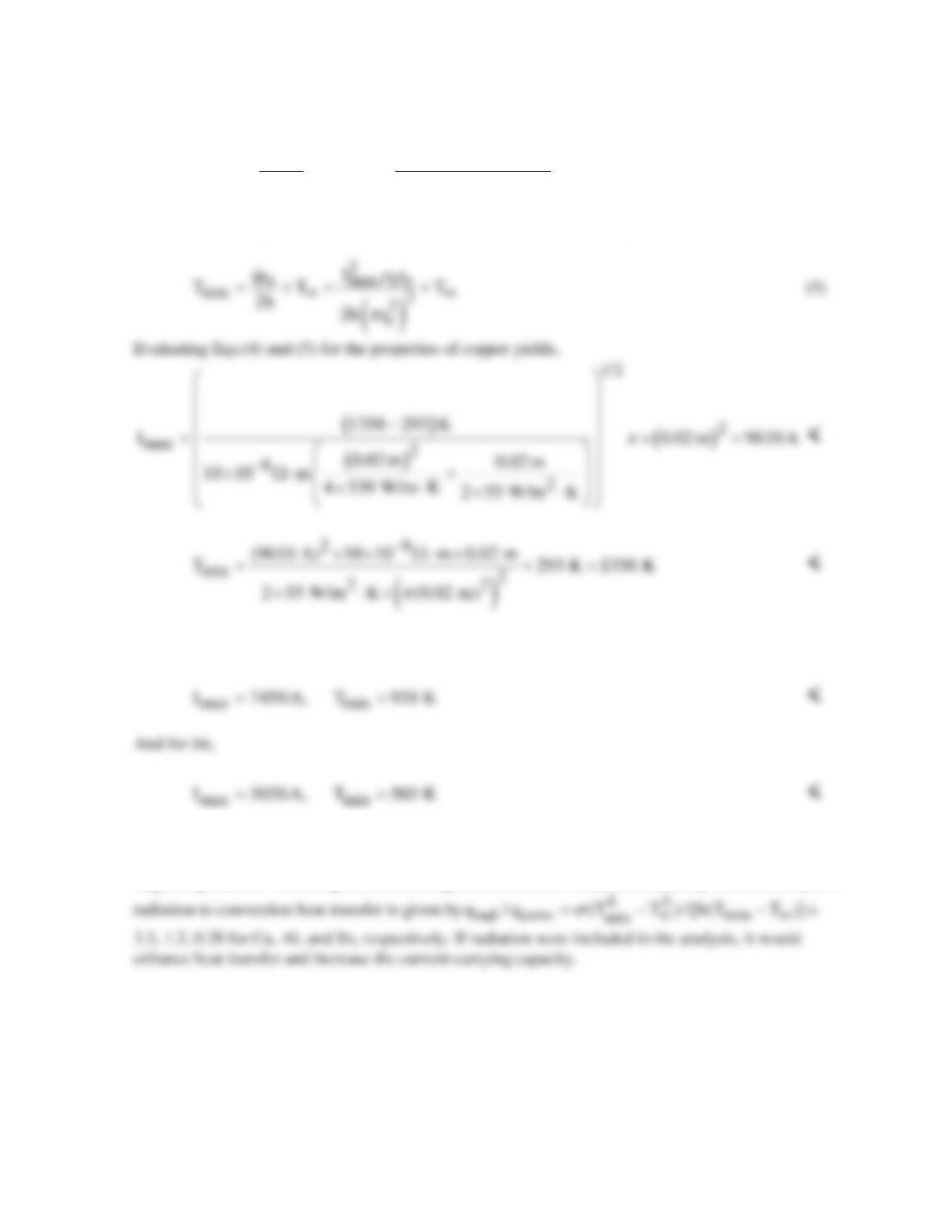
SCHEMATIC:
ASSUMPTIONS: (1) Steady-state, (2) Constant properties, (3) Negligible radiation exchange with
surroundings.
PROPERTIES: Given, Cu:
e
ρ
= 10 × 10-8 W⋅m, Al:
e
ρ
= 10 × 10-8 W⋅m, Sn:
e
ρ
= 20 × 10-8 W⋅m.
Table A.1, Cu: Tm = 1358 K, k = 339 W/m⋅K; Al: Tm = 933 K, k = 218 W/m⋅K; Sn: Tm = 505 K, k =
62.2 W/m⋅K. Thermal conductivities have been evaluated at highest available temperature.
ANALYSIS: The maximum temperature should not exceed the melting temperature of the material.
The maximum temperature occurs at the centerline and can be found from Equation 3.58 evaluated at
r = 0. The surface temperature can be related to the known environment temperature through Equation
3.60. Thus,
Continued…
PROBLEM 3.63 (Cont.)
()
1/ 2
1/ 2
22
max max
max o o
2
eeo o
q TT
Ir r
r / 4k r / 2h
ππ
ρρ
∞
−
= =
+
(4)
The minimum temperature occurs at the surface of the cable, so from Equation 3.60,
Similarly for aluminum,
COMMENTS: (1) The minimum (surface) temperature is almost equal to the maximum (melting)
temperature; the cable is nearly isothermal. (2) The neglect of radiation is a poor assumption for such
large temperatures. Assuming the surroundings are also at 293 K and the emissivity is one, the ratio of
PROBLEM 3.64
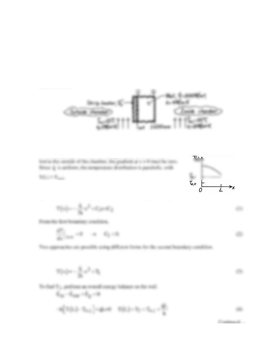
KNOWN: Wall of thermal conductivity k and thickness L with uniform generation
q
; strip heater
with uniform heat flux
o
q;
′′
prescribed inside and outside air conditions (hi, T∞,i, ho, T∞,o).
FIND: (a) Sketch temperature distribution in wall if none of the heat generated within the wall is lost
to the outside air, (b) Temperatures at the wall boundaries T(0) and T(L) for the prescribed condition,
(c) Value of
′′
q
o
required to maintain this condition, (d) Temperature of the outer surface, T(L), if
o
q=0 but q′′
corresponds to the value calculated in (c).
SCHEMATIC:
ASSUMPTIONS: (1) Steady-state conditions, (2) One-dimensional conduction, (3) Uniform
volumetric generation, (4) Constant properties.
ANALYSIS: (a) If none of the heat generated within the wall is
(b) To find temperatures at the boundaries of wall, begin with the
general solution to the appropriate form of the heat equation (Eq.3.40).
Approach No. 1: With boundary condition
( )
1
T0 T→=
Continued …
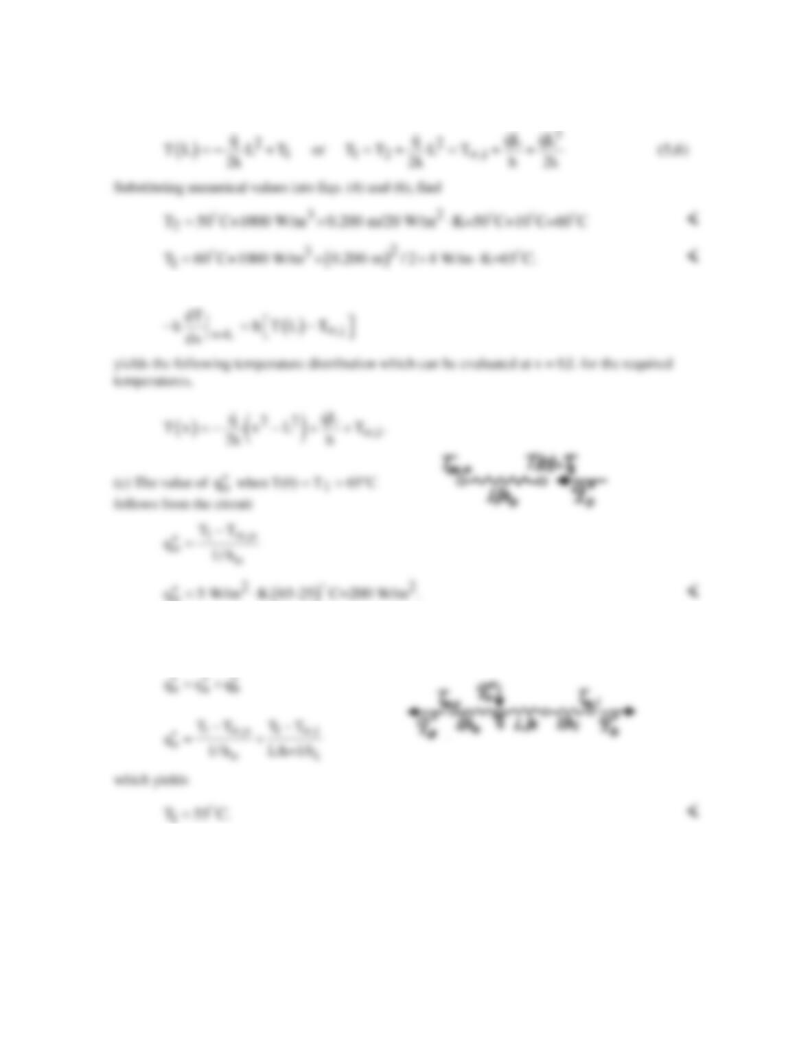
PROBLEM 3.64 (Cont.)
and from Eq. (3) with x = L and T(L) = T2,
Approach No. 2: Using the boundary condition
o
(d) With
q=0,
the situation is represented
by the thermal circuit shown. Hence,
PROBLEM 3.65
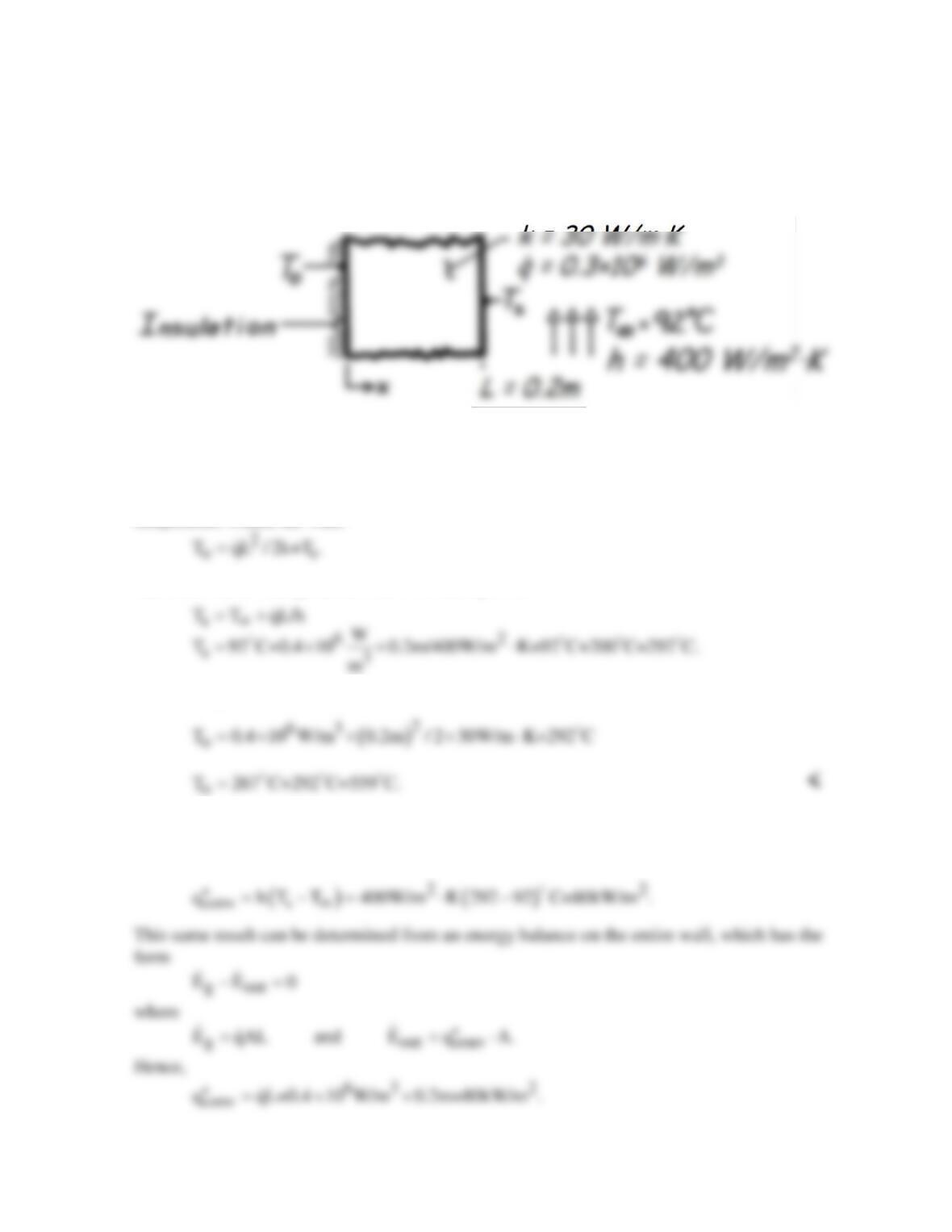
KNOWN: Plane wall with internal heat generation which is insulated at the inner surface and
subjected to a convection process at the outer surface.
FIND: Maximum temperature in the wall.
SCHEMATIC:
ASSUMPTIONS: (1) Steady-state conditions, (2) One-dimensional conduction with uniform
volumetric heat generation, (3) Inner surface is adiabatic.
ANALYSIS: The temperature at the inner surface is given by Eq. 3.48 and is the maximum
temperature within the wall,
The outer surface temperature follows from Eq. 3.51,
It follows that
COMMENTS: The heat flux leaving the wall can be determined from knowledge of h, Ts
and T∞ using Newton’s law of cooling.
PROBLEM 3.66
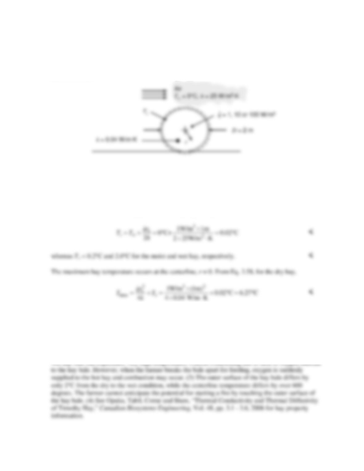
KNOWN: Diameter, thermal conductivity and microbial energy generation rate in cylindrical hay
bales. Ambient conditions.
FIND: The maximum hay temperature for
q
= 1, 10, and 100 W/m3.
SCHEMATIC:
ASSUMPTIONS: (1) Steady–state conditions, (2) Constant properties, (3) One-dimensional heat
transfer (4) Uniform volumetric generation, (5) Negligible radiation, (6) Negligible conduction to or
from the ground.
PROPERTIES: k = 0.04 W/m⋅K (given).
ANALYSIS: The surface temperature of the dry hay is (Eq. 3.60)
whereas Tmax = 62.7°C and 627°C for the moist and wet hay, respectively. <
COMMENTS: (1) The hay begins to lose its nutritional value at temperatures exceeding 50°C.
Therefore the center of the moist hay bale will lose some of its nutritional value. (2) The center of the
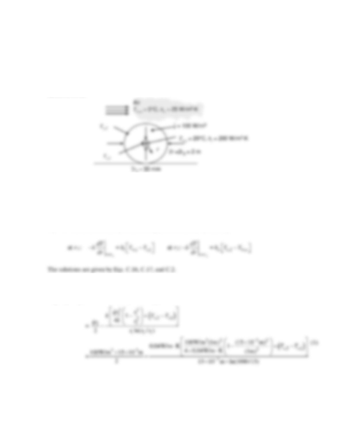
PROBLEM 3.67
KNOWN: Diameter, thermal conductivity and microbial energy generation rate in cylindrical hay
bales. Thin-walled tube diameter and insertion location. Temperature of flowing water and convective
heat transfer coefficient inside the tube. Ambient conditions.
FIND: (a) Steady–state heat transfer to the water per unit length of tube, (b) Plot of the radial
temperature distribution, T(r), in the hay (c) Plot of the heat transfer to the water per unit length of
tube for bale diameters of 0.2 m ≤ D ≤ 2 m for
q
= 100 W/m3.
SCHEMATIC:
ASSUMPTIONS: (1) Steady–state conditions, (2) Constant properties, (3) One-dimensional heat
transfer (4) Uniform volumetric generation, (5) Negligible radiation, (6) Negligible conduction to or
from the ground.
PROPERTIES: k = 0.04 W/m⋅K (given).
ANALYSIS: (a) The temperature distribution is found by utilizing the general solution given by
Eq. 3.56 with mixed boundary conditions applied at r1 and r2. Specifically,
From Eq. C.16,
2
, , ,1
( ) 200 W/m K (20 C T )
i i s s ,1
hT T
∞∞
− = ⋅ × °−
Continued…
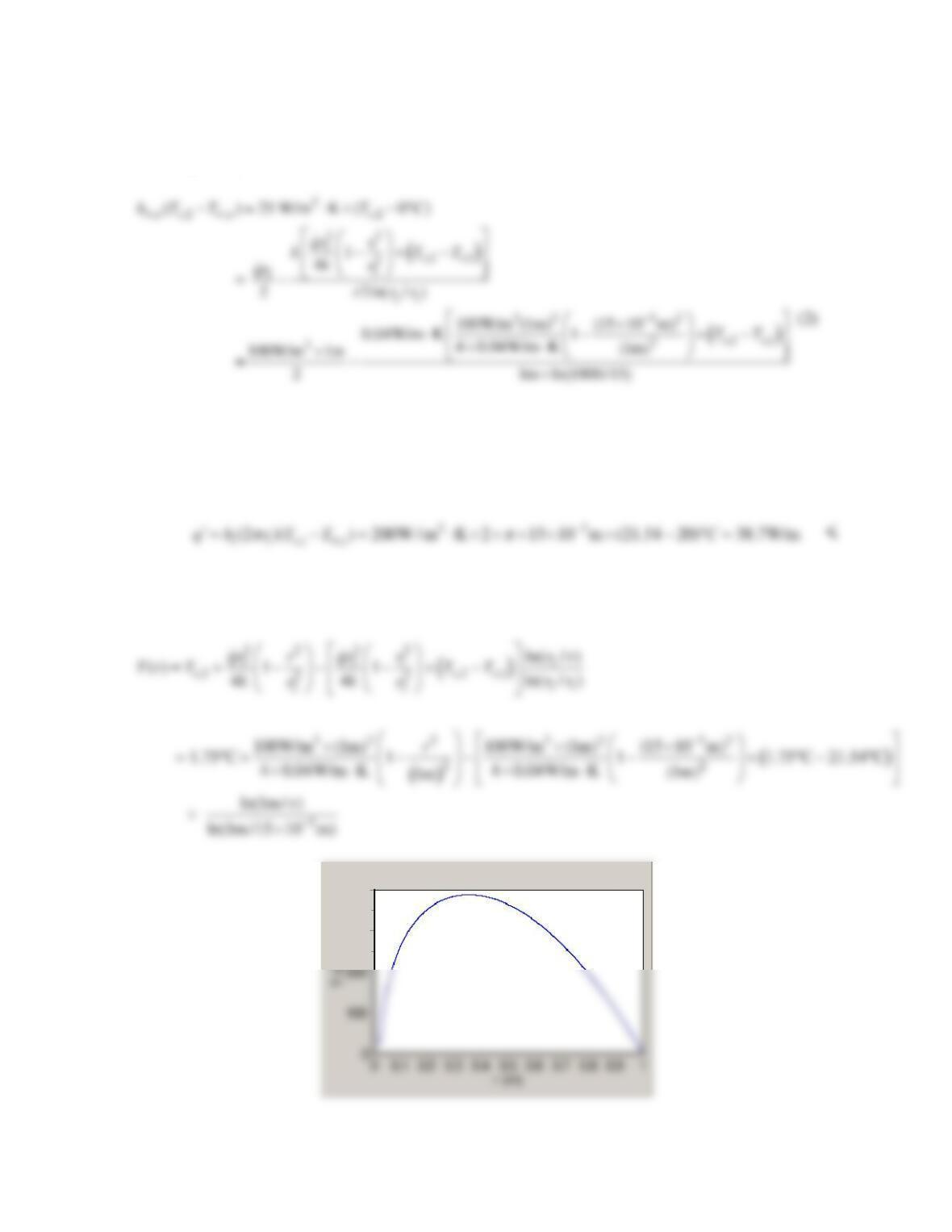
PROBLEM 3.67 (Cont.)
From Eq. C.17,
Equations (1) and (2) may be solved simultaneously to yield Ts,1 = 21.54°C, Ts,2 = 1.75°C. The heat
transfer to the cold fluid per unit length is
(b) The radial temperature distribution is evaluated from Eq. C.2 and is shown below.
400
300
Continued…
PROBLEM 3.67 (Cont.)
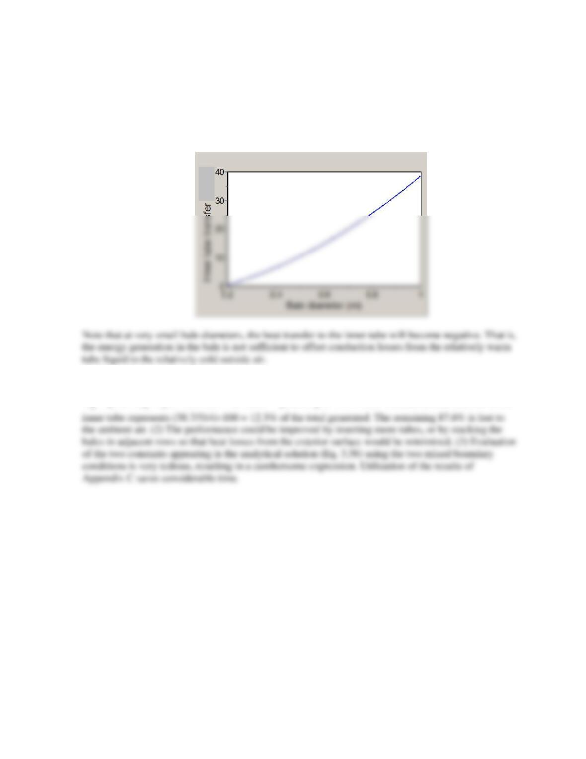
Note that the maximum temperature occurs at r ≈ 0.35 m.
(c) The rate of heat transfer to the cool fluid, per unit length, is shown versus the bale diameter in the
plot below.
COMMENTS: (1) The energy generated in the bale per unit length is
( )
2
‘ 22 3 2
21
( ) 100W/m (1m 0.015m ) 314 W/m.
g
E q rr
ππ
=×× − = ×× − =
Hence, the heat transfer to the
(W/m)
PROBLEM 3.68
KNOWN: Composite wall with outer surfaces exposed to convection process.
FIND: (a) Volumetric heat generation and thermal conductivity for material B required for special
conditions, (b) Plot of temperature distribution, (c) T1 and T2, as well as temperature distributions
corresponding to loss of coolant condition where h = 0 on surface A.
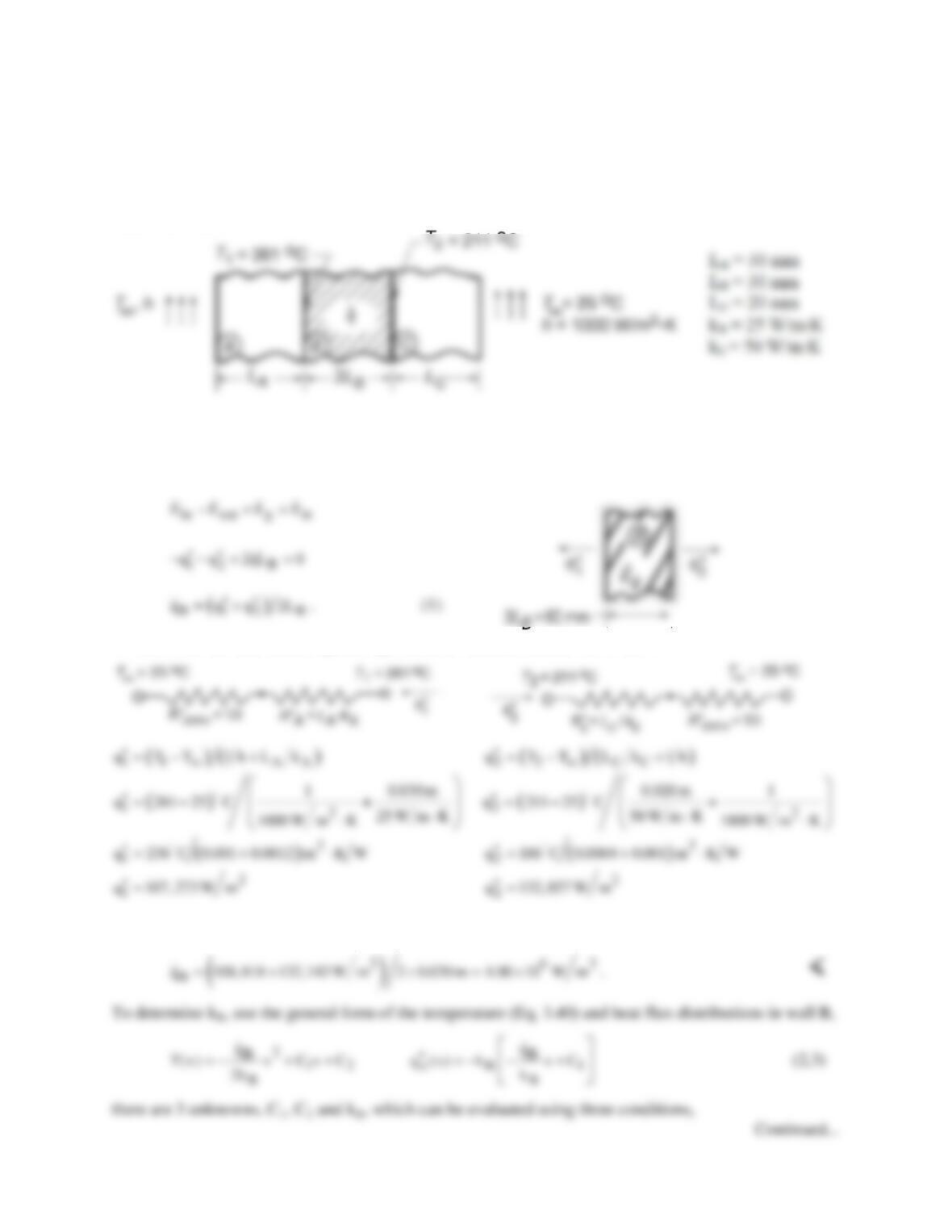
SCHEMATIC:
ASSUMPTIONS: (1) Steady-state, one-dimensional heat transfer, (2) Negligible contact resistance at
interfaces, (3) Uniform generation in B; zero in A and C.
ANALYSIS: (a) From an energy balance on wall B,
To determine the heat fluxes,
¢¢
q
1
and
¢¢
q
2
, construct thermal circuits for A and C:
Using the values for
1
q′′
and
2
q′′
in Eq. (1), find
PROBLEM 3.68 (Cont.)
( ) ( )
2
B
B 1 B 1B 2
B
q
T L T L CL C
2k
−==− − − +
where T1 = 261°C (4)
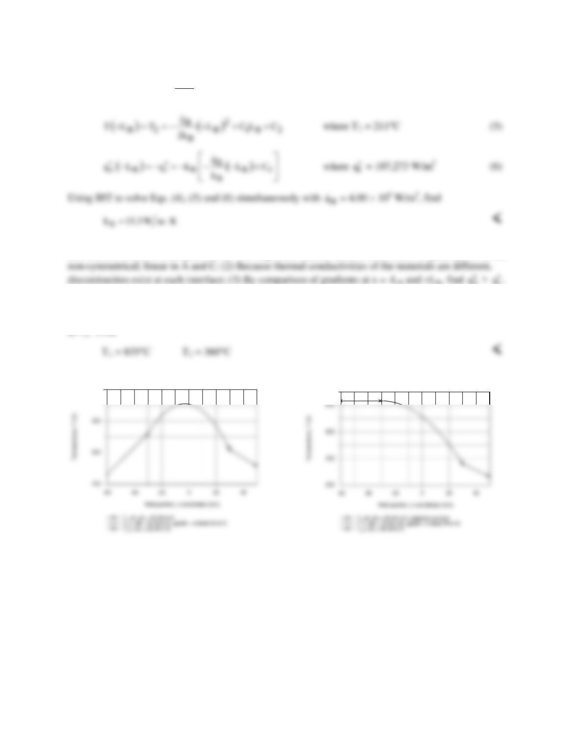
(b) Following the method of analysis in the IHT Example 3.6, User-Defined Functions, the temperature
distribution is shown in the plot below. The important features are (1) Distribution is quadratic in B, but
2
1
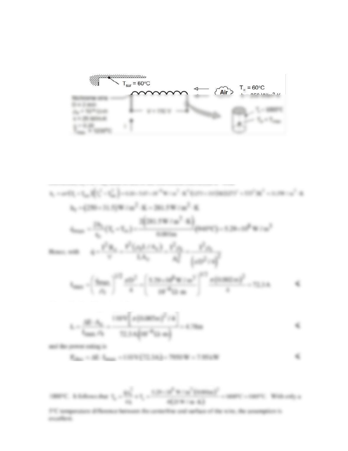
(c) Using the same method of analysis as for Part (c), the temperature distribution is shown in the plot
below when h = 0 on the surface of A. Since the left boundary is adiabatic, material A will be isothermal
at T1. Find
400
Loss of coolant on surface A
1
PROBLEM 3.69
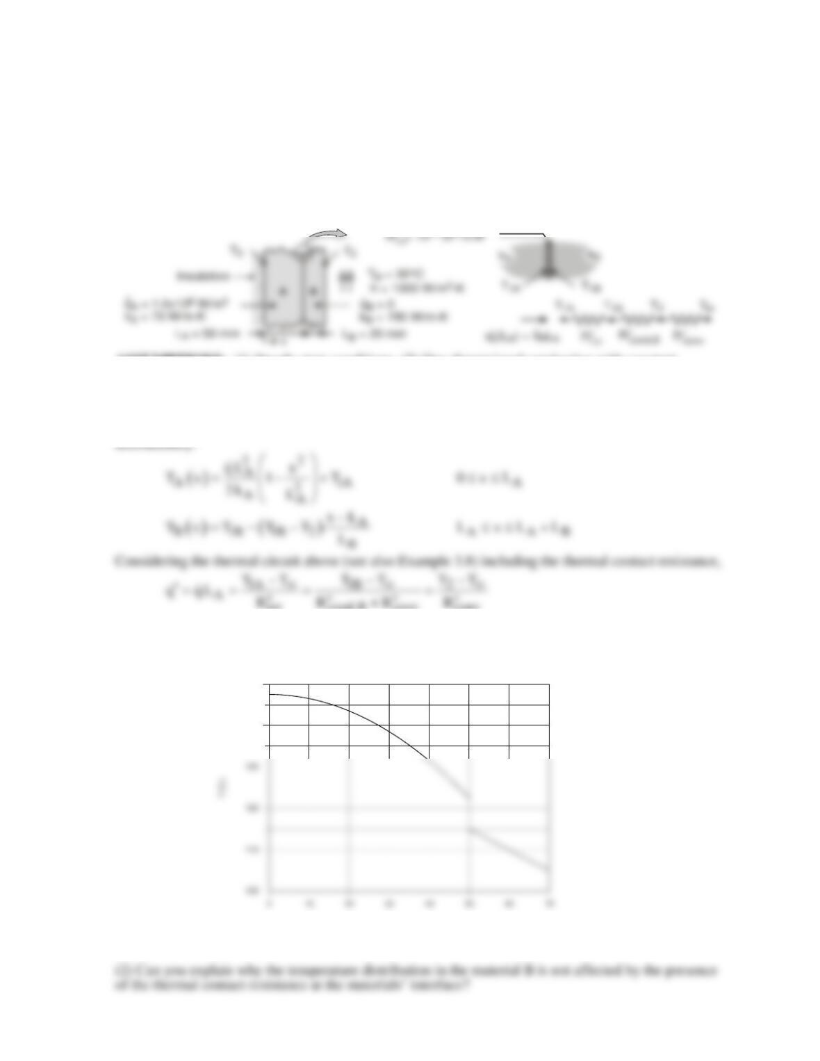
KNOWN: Diameter, resistivity, thermal conductivity, emissivity, voltage, and maximum temperature
of heater wire. Convection coefficient and air exit temperature. Temperature of surroundings.
FIND: Maximum operating current, heater length and power rating.
SCHEMATIC:
ASSUMPTIONS: (1) Steady-state, (2) Uniform wire temperature, (3) Constant properties, (4)
Radiation exchange with large surroundings.
ANALYSIS: Assuming a uniform wire temperature, Tmax = T(r = 0) ≡ To ≈ Ts, the maximum
volumetric heat generation may be obtained from Eq. (3.60), but with the total heat transfer
Also, with ∆E = I Re = I (ρeL/Ac),
elec max
COMMENTS: To assess the validity of assuming a uniform wire temperature, Eq. (3.58) may be
used to compute the centerline temperature corresponding to
max
q
and a surface temperature of
PROBLEM 3.70
KNOWN: Composite wall of materials A and B. Wall of material A has uniform generation, while
wall B has no generation. The inner wall of material A is insulated, while the outer surface of
material B experiences convection cooling. Thermal contact resistance between the materials is
42
t,c
R 10 m K / W
−
′′ = ⋅
. See Example 3.7 that considers the case without contact resistance.
FIND: Compute and plot the temperature distribution in the composite wall.
SCHEMATIC:
ASSUMPTIONS: (1) Steady–state conditions, (2) One-dimensional conduction with constant
properties, and (3) Inner surface of material A is adiabatic.
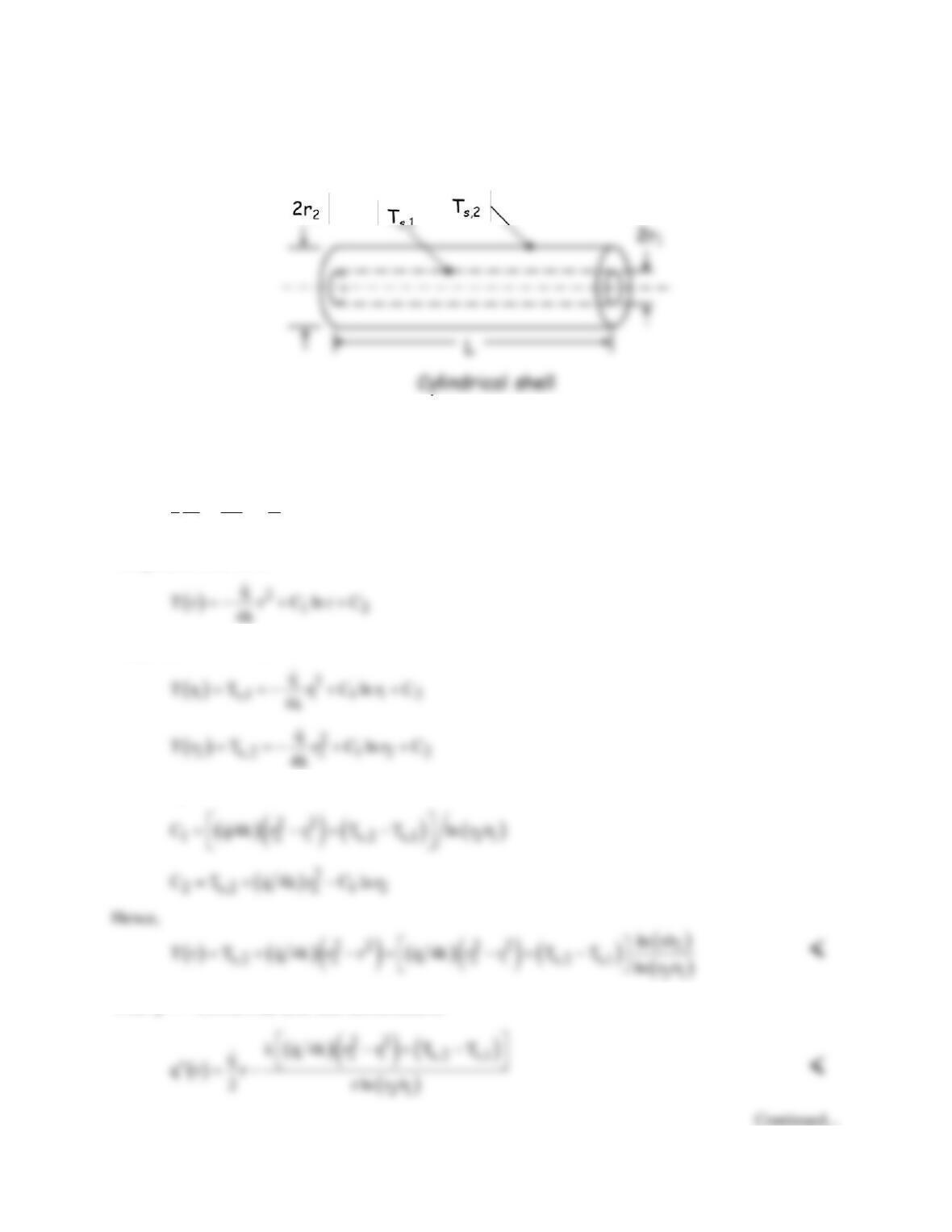
ANALYSIS: From the analysis of Example 3.8, we know the temperature distribution in material A
is parabolic with zero slope at the inner boundary, and that the distribution in material B is linear. At
the interface between the two materials, x = LA, the temperature distribution will show a
tot cond,B conv conv
find TA(0) = 147.5°C, T1A = 122.5°C, T1B = 115°C, and T2 = 105°C. Using the foregoing equations
in IHT, the temperature distributions for each of the materials can be calculated and are plotted on the
graph below.
COMMENTS: (1) The effect of the thermal contact resistance between the materials is to increase
the maximum temperature of the system.
Effect of thermal contact resistance on temperature distribution
x (m m )
140
150
PROBLEM 3.71
KNOWN: Cylindrical shell with uniform heat generation and surface temperatures.
FIND: Radial distributions of temperature, heat flux, and heat rate.
SCHEMATIC:
ASSUMPTIONS: (1) One-dimensional, steady-state conduction, (2) Uniform heat generation, (3)
Constant k.
ANALYSIS: For the cylindrical shell, the appropriate form of the heat equation is
1 d dT q
r0
r dr dr k
+=
The general solution is
Applying the boundary conditions, it follows that
which may be solved for
With
q k dT/dr
′′ = −
, the heat flux distribution is
Continued…