PROBLEM 3.29
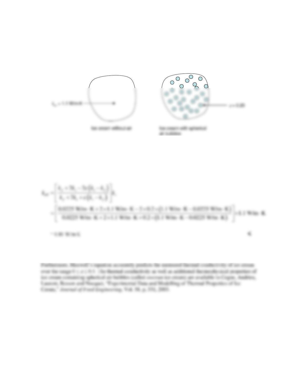
KNOWN: Thermal conductivity of ice cream containing no air at T = -20°C. Shape and volume
fraction of air bubbles.
FIND: The thermal conductivity of commercial ice cream characterized by
e
= 0.20 at T = –20°C.
SCHEMATIC:
ASSUMPTIONS: (1) Constant properties, (2) Spherical air bubbles.
PROPERTIES: Table A.4, Air (300 K): kair = 0.0225 W/m∙K.
ANALYSIS: Maxwell’s expression for the effective thermal conductivity may be used, with kf = kair
and ks = kna. Hence,
COMMENTS: (1) The reduction in the effective thermal conductivity due to the presence of the air
bubbles is 26%. (2) The predicted thermal conductivity is in good agreement with measured values.
PROBLEM 3.30
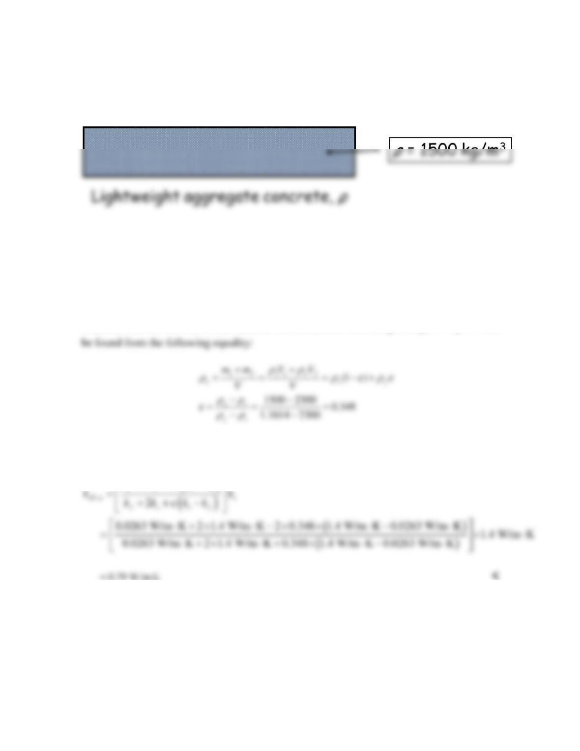
KNOWN: Density of stone mix concrete slab, within which are small spherical pockets of air.
FIND: Thermal conductivity of the aggregate.
SCHEMATIC:
ASSUMPTIONS: (1) Constant properties.
PROPERTIES: Table A.3 (T = 300 K): Stone mix concrete; ks = 1.4 W/m⋅K,
ρ
s= 2300 kg/m3, cp,s =
880 J/kg⋅K. Table A.4 (T = 300 K): Air; kf = 0.0263 W/m⋅K,
ρ
f = 1.1614 kg/m3, cp,f = 1007 J/kg⋅K.
ANALYSIS: The density of the aggregate,
ρ
a, is equal to its mass divided by its volume,
where the mass is the sum of the concrete and air masses. Thus the porosity,
/,
f
VV
e
=
can
Once the porosity is known, the effective thermal conductivity can be found from Maxwell’s
expression, Eq. 3.25. Hence,
( )
22
f s sf
k k kk
e
+− −
= 0.79 W/m∙K <
COMMENT: The thermal conductivity and density are reduced significantly relative to the stone
mix concrete values.
PROBLEM 3.31
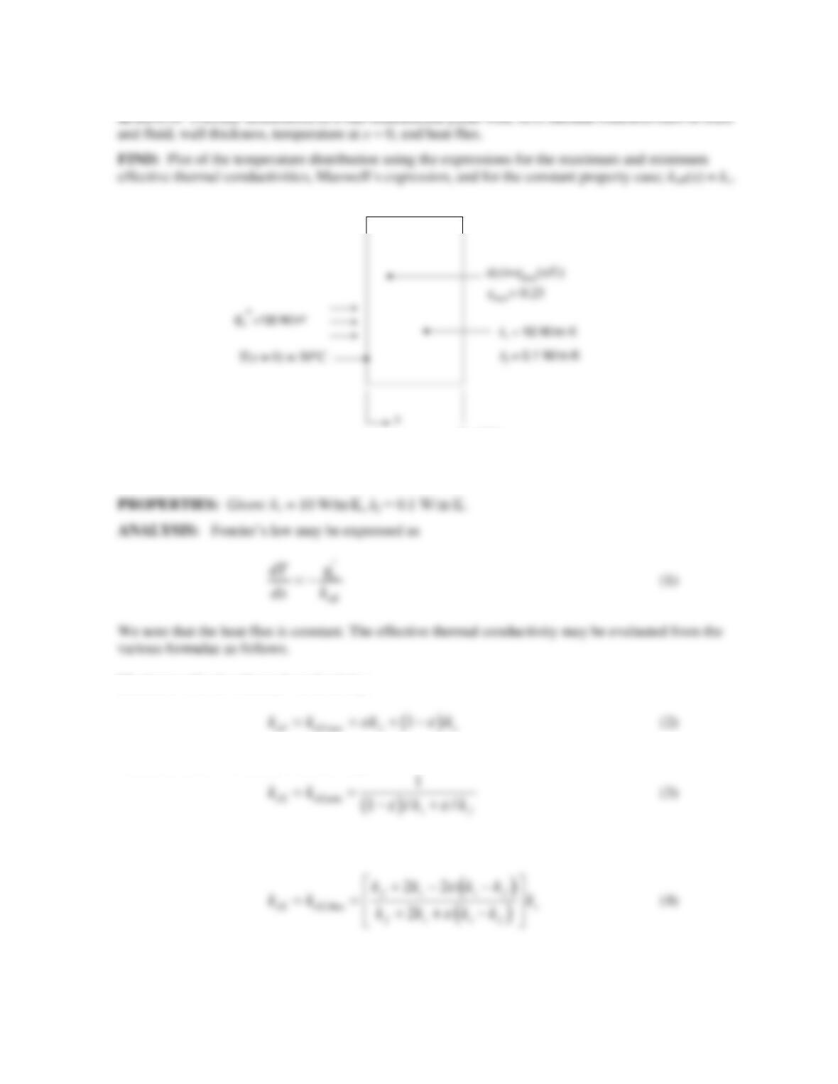
SCHEMATIC:
ASSUMPTIONS: (1) Constant properties within the two phases, (2) Negligible radiation, (3) No
thermal energy generation, (4) Steady state, one–dimensional heat transfer.
Maximum effective thermal conductivity:
Minimum effective thermal conductivity:
Maxwell’s expression:
Continued…
L = 1 m
PROBLEM 3.31 (Cont.)
No dispersed phase:
eff s
kk=
(5)
Equations 2, 3, 4, or 5 may be substituted into Equation 1 and the expression may be integrated
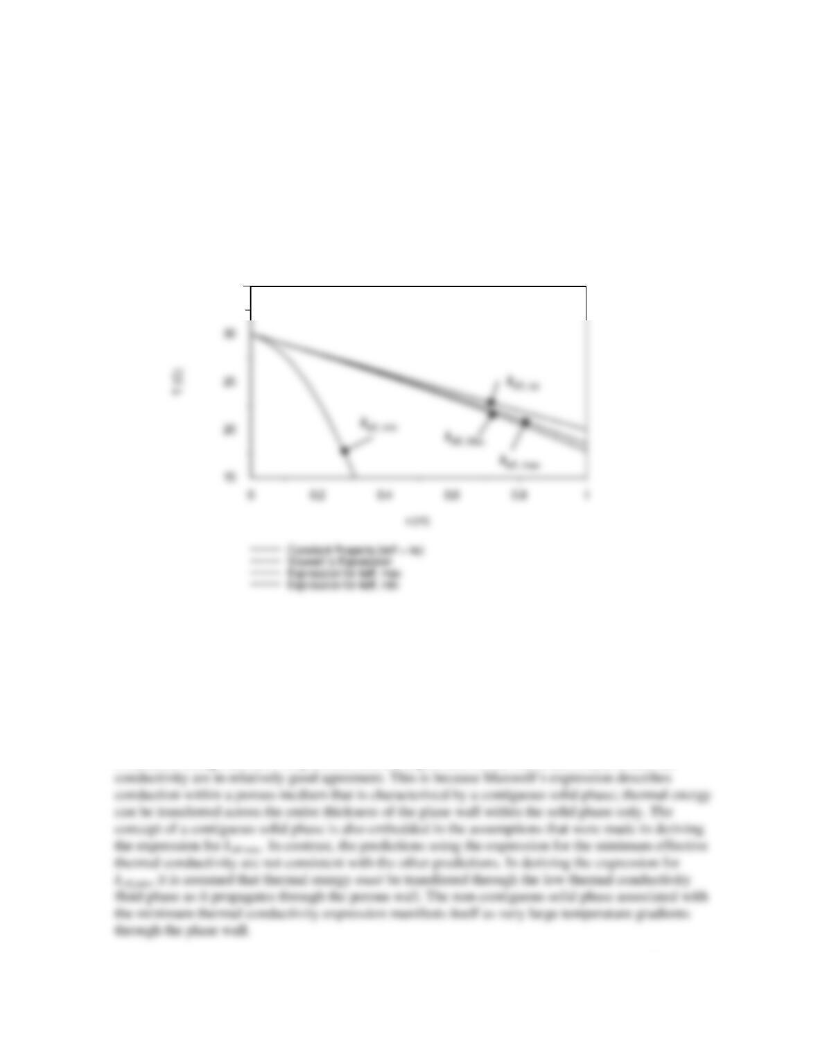
numerically using a commercial code. IHT was used to generate the following temperature
distributions.
The constant property solution exhibits a linear temperature distribution.
The introduction of the low thermal conductivity matter within the medium decreases its effective
thermal conductivity. From Equation (1), the temperature gradient must become larger in order to
sustain the imposed heat flux as the effective thermal conductivity decreases. The increased
temperature gradients are evident in the plot.
Predictions using Maxwell’s expression, and the expression for the maximum effective thermal
Continued…
Temperatur e Distribution T(x)
35
PROBLEM 3.31 (Cont.)
COMMENTS: (1) It is important to be cognizant of the morphology of the porous medium before
selecting the appropriate expression for the effective thermal conductivity. (2) The IHT code is shown
below.
//Input phase properties, dimensions, thermal boundary condition, and porosity parameter.
ks = 10 //W/mK
kf = 0.1 //W/mK
PROBLEM 3.32
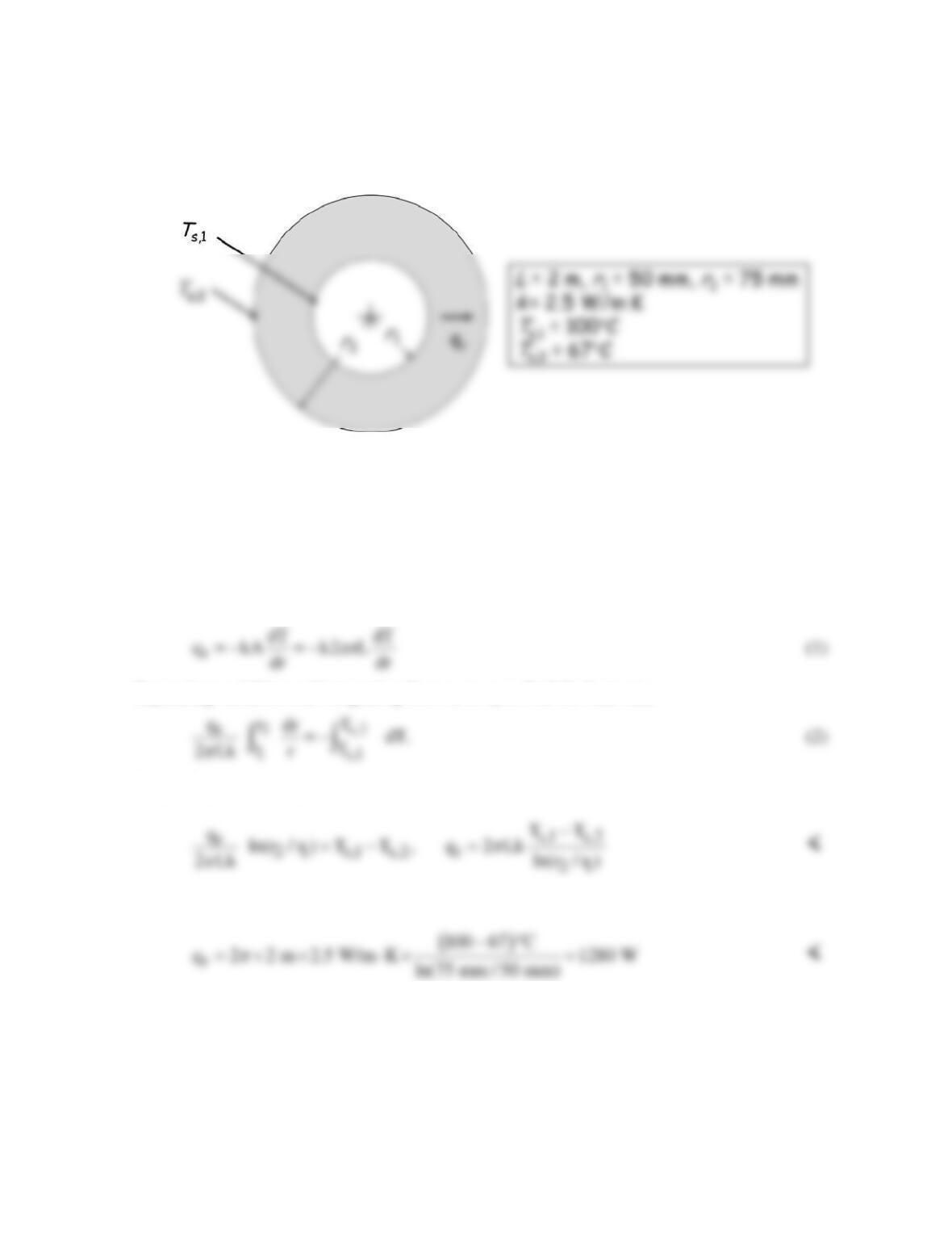
KNOWN: Conduction in a hollow cylinder with known dimensions and properties.
FIND: Expression for the radial heat rate and its value for given conditions.
SCHEMATIC:
ASSUMPTIONS: (1) Steady–state conditions, (2) One-dimensional conduction in r-
direction, (3) No internal heat generation, (4) Constant properties.
PROPERTIES: Given, k= 2.5 W/m⋅K.
ANALYSIS: Based upon the assumptions, and following similar methodology to Example
3.5, qr is a constant independent of r and the area normal to the direction of heat flow is
A 2 rL
π
=
. Accordingly,
Separating variables and integrating from r1 to r2 to find the heat rate,
Integrating and solving for qr,
Evaluating the expression for qr under the given conditions yields
COMMENTS: (a) The expression for the heat rate agrees with Equation 3.32, as it must. (b)
If the temperature distribution were desired, the integration in Eq. (2) could now be repeated
using integration to arbitrary upper limits r and T(r).
PROBLEM 3.33
KNOWN: Conduction in a conical section with prescribed diameter, D, as a function of x in
the form D = ax1/2.
FIND: (a) Temperature distribution, T(x), (b) Heat transfer rate, qx.
SCHEMATIC:
ASSUMPTIONS: (1) Steady-state conditions, (2) One-dimensional conduction in x-
direction, (3) No internal heat generation, (4) Constant properties.
PROPERTIES: Table A-1, Pure Aluminum (500K): k= 236 W/m⋅K.
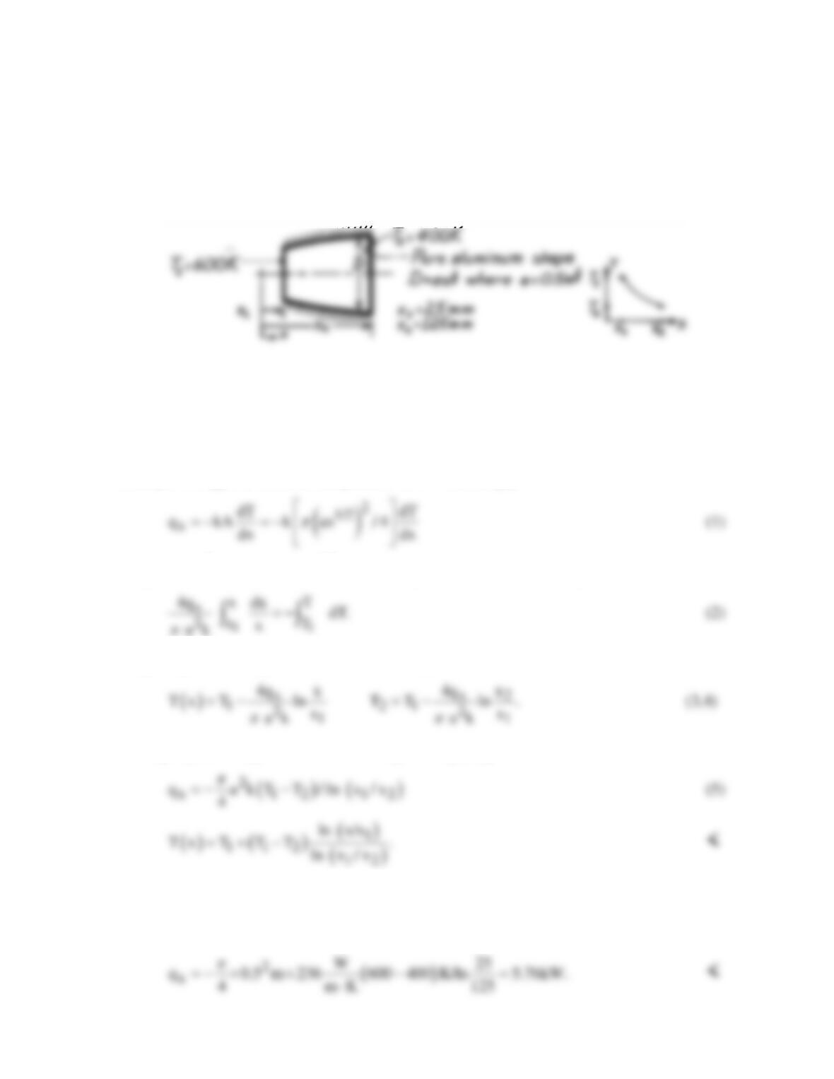
ANALYSIS: (a) Based upon the assumptions, and following the same methodology of
Example 3.4, qx is a constant independent of x. Accordingly,
using A = πD2/4 where D = ax1/2. Separating variables and identifying limits,
Integrating and solving for T(x) and then for T2,
Solving Eq. (4) for qx and then substituting into Eq. (3) gives the results,
From Eq. (1) note that (dT/dx)⋅x = Constant. It follows that T(x) has the distribution shown
above.
(b) The heat rate follows from Eq. (5),
PROBLEM 3.34
KNOWN: Geometry and surface conditions of a truncated solid cone.
FIND: (a) Temperature distribution, (b) Rate of heat transfer across the cone.
SCHEMATIC:
ASSUMPTIONS: (1) Steady-state conditions, (2) One-dimensional conduction in x, (3)
Constant properties.
PROPERTIES: Table A-1, Aluminum (333K): k = 238 W/m⋅K.
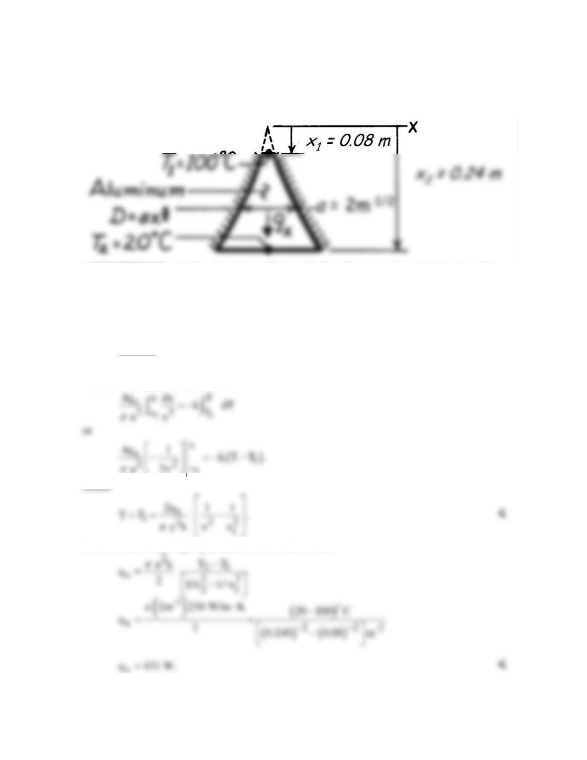
ANALYSIS: (a) From Fourier’s law, Eq. 2.1, with
()
2 23
A= D /4 a /4 x ,
ππ
=
it follows that
x
23
4q dx kdT.
ax
π
= −
Hence, since qx is independent of x,
(b) From the foregoing expression, it also follows that
COMMENTS: The foregoing results are approximate due to use of a one-dimensional model
in treating what is inherently a two-dimensional problem.
PROBLEM 3.35
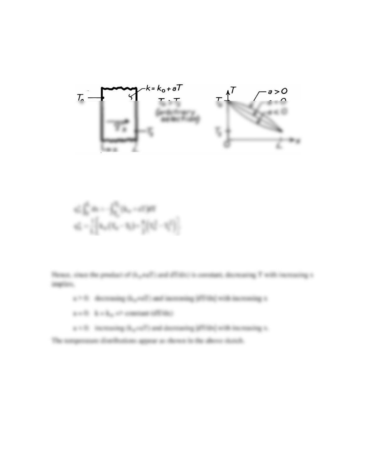
KNOWN: Temperature dependence of the thermal conductivity, k.
FIND: Heat flux and form of temperature distribution for a plane wall.
SCHEMATIC:
ASSUMPTIONS: (1) One-dimensional conduction through a plane wall, (2) Steady–state
conditions, (3) No internal heat generation.
ANALYSIS: For the assumed conditions, qx and A(x) are constant and Eq. 3.26 gives
From Fourier’s law,
( )
xo
q k aT dT/dx.
′′ =−+
PROBLEM 3.36
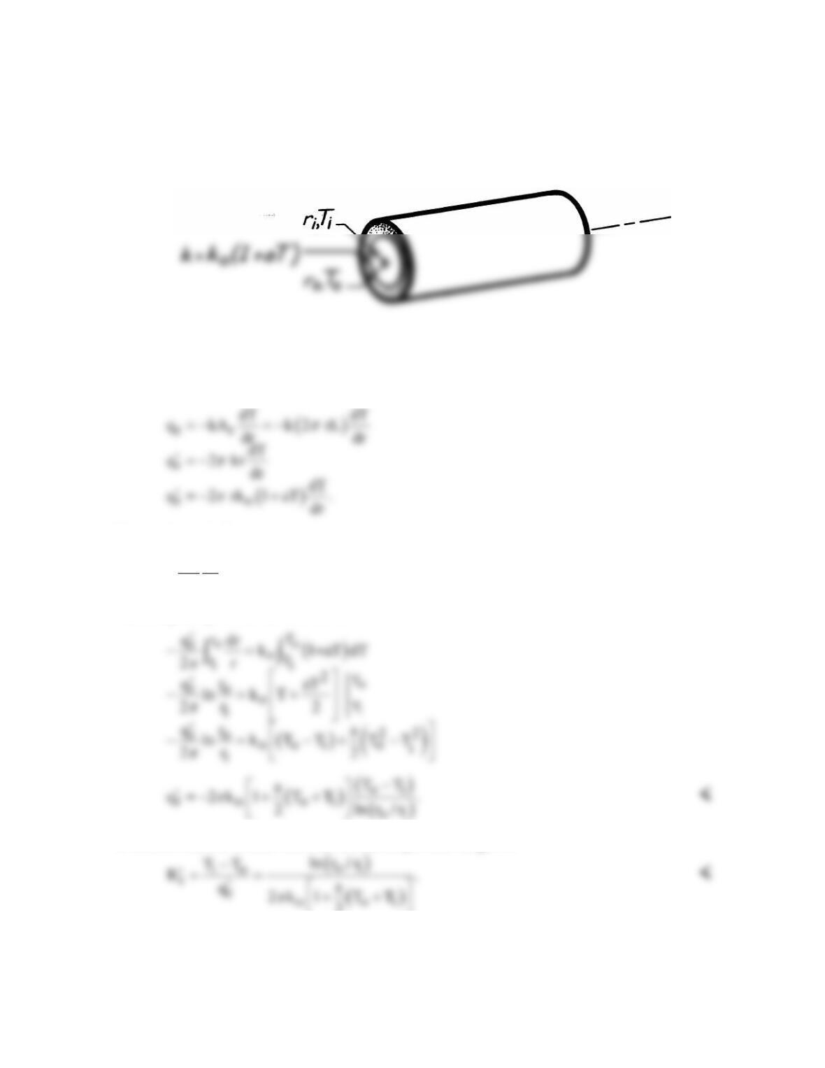
KNOWN: Temperature dependence of tube wall thermal conductivity.
FIND: Expressions for heat transfer per unit length and tube wall thermal (conduction)
resistance.
SCHEMATIC:
ASSUMPTIONS: (1) Steady-state conditions, (2) One-dimensional radial conduction, (3)
No internal heat generation.
ANALYSIS: From Eq. 3.29, the appropriate form of Fourier’s law is
Separating variables,
( )
ro
q dr k 1 aT dT
2r
π
′
−=+
and integrating across the wall, find
It follows that the overall thermal resistance per unit length is
2
COMMENT: Note the necessity of the stated assumptions to treating
r
q′
as independent of r.
PROBLEM 3.37
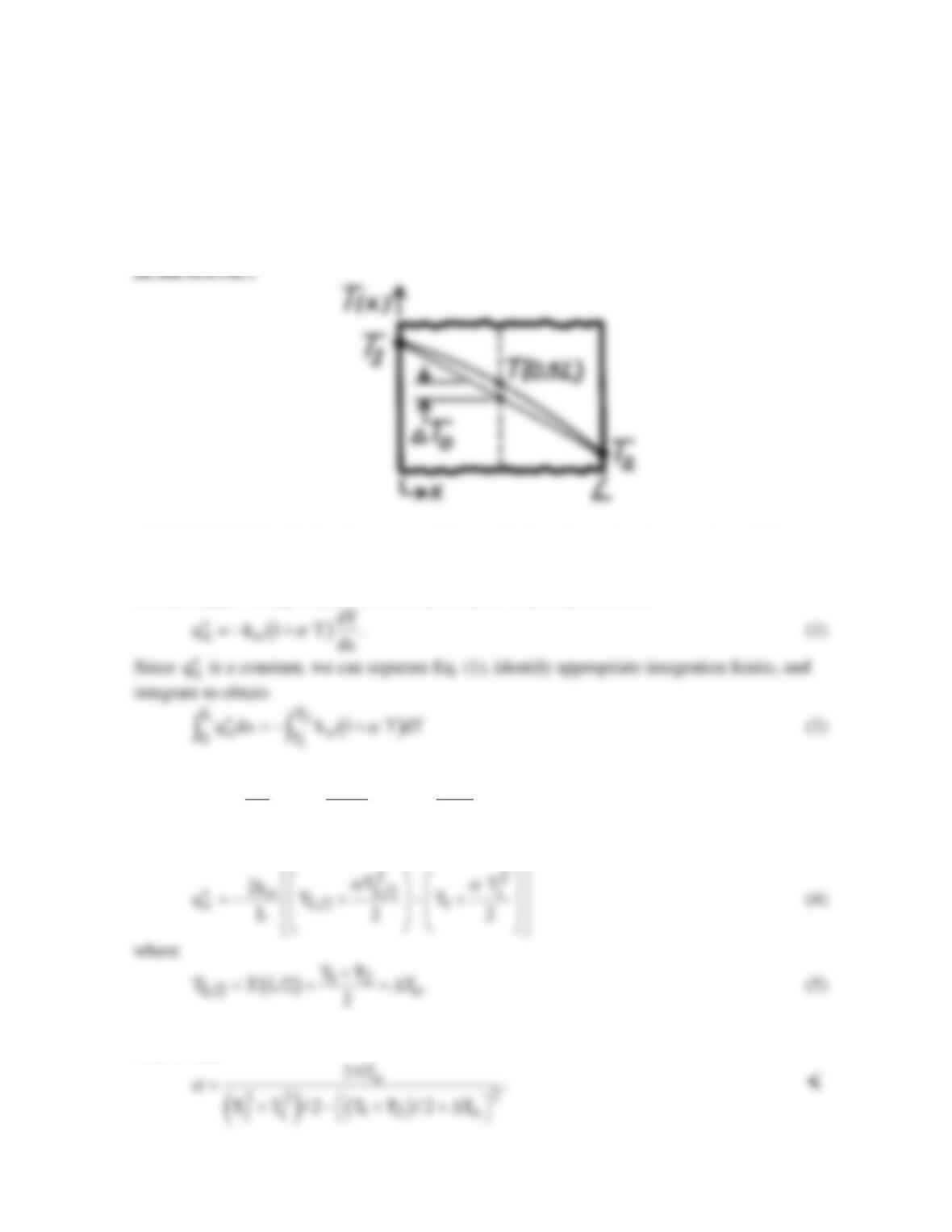
KNOWN: Steady-state temperature distribution of convex shape for material with k = ko(1 +
αT) where α is a constant and the mid-point temperature is ∆To higher than expected for a
linear temperature distribution.
FIND: Relationship to evaluate α in terms of ∆To and T1, T2 (the temperatures at the
boundaries).
ASSUMPTIONS: (1) Steady-state conditions, (2) One-dimensional conduction, (3) No
internal heat generation, (4) α is positive and constant.
ANALYSIS: At any location in the wall, Fourier’s law has the form
22
o21
x2 1
TT
k
q T T.
L2 2
αα
′′ =− + −+
(3)
We could perform the same integration, but with the upper limits at x = L/2, to obtain
Setting Eq. (3) equal to Eq. (4), substituting from Eq. (5) for TL/2, and solving for α, it
follows that
PROBLEM 3.38
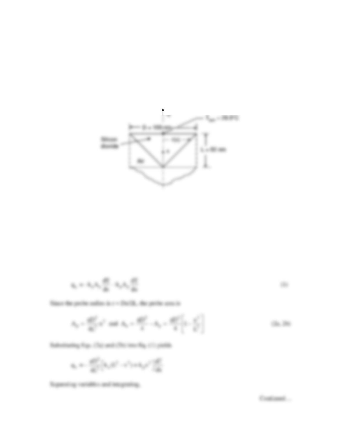
KNOWN: Construction and dimensions of a device to measure the temperature of a surface.
Ambient and sensing temperatures, and thermal resistance between the sensing element and the
pivot point.
FIND: (a) Thermal resistance between the surface temperature and the sensing temperature, (b)
Surface temperature for Tsen = 28.5°C.
SCHEMATIC:
ASSUMPTIONS: (1) Steady-state conditions, (2) One-dimensional heat transfer, (3) Negligible
nanoscale effects, (4) Constant properties.
PROPERTIES: Table A.2, polycrystalline silicon dioxide (300 K): k = 1.38 W/m⋅K. Table A.4,
air (300 K): k = 0.0263 W/m⋅K.
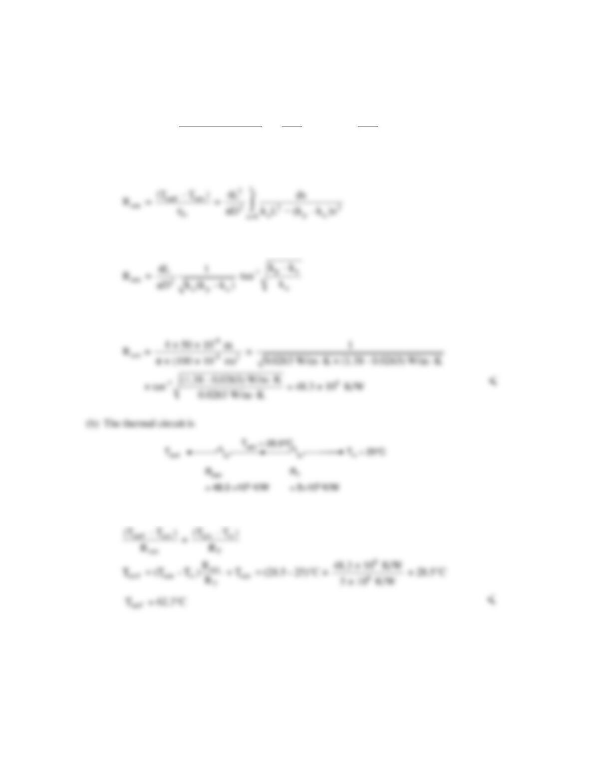
ANALYSIS:
(a) At any x location, heat transfer in the x-direction occurs by conduction in the air as well as
conduction in the probe. Applying Fourier’s law,
PROBLEM 3.38 (Cont.)
( )
sen
surf
T
L22
x sen surf
22 2 2 2
ap
x=0 T=T
dx πD πD
q = – dT = – T – T
k (L – x ) + k x 4L 4L
∫∫
Therefore, the thermal resistance associated with the probe is
Carrying out the integration yields
Substituting values gives
Hence,
COMMENT: Heat transfer within the probe region will not be one–dimensional and
modification of heat transfer due to nanoscale effects may be important. However, the probe may
be calibrated by measuring the surface temperature of a large isothermal object.
PROBLEM 3.39
KNOWN: Thickness and inner surface temperature of calcium silicate insulation on a steam pipe.
Convection and radiation conditions at outer surface.
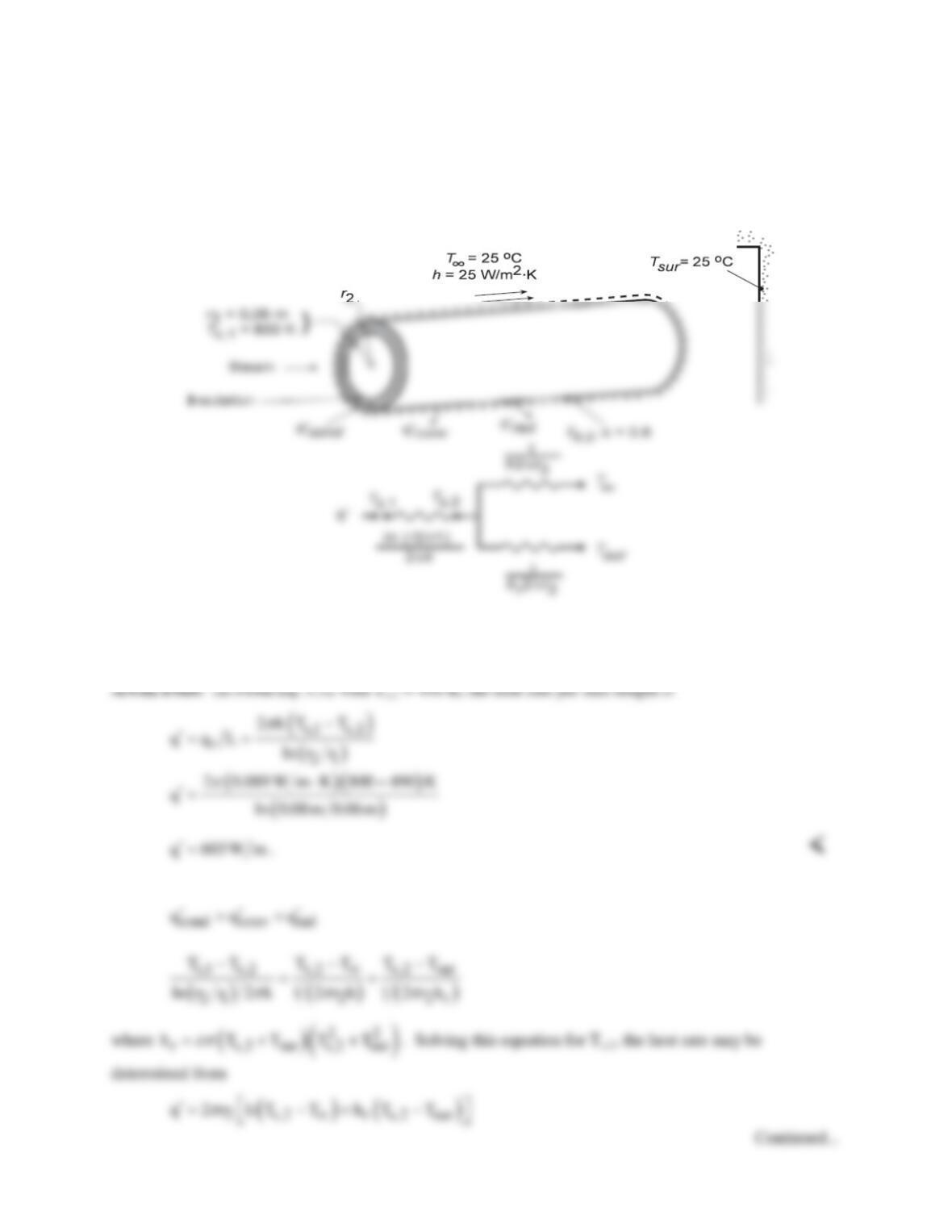
FIND: (a) Heat loss per unit pipe length for prescribed insulation thickness and outer surface
temperature. (b) Heat loss and radial temperature distribution as a function of insulation thickness.
SCHEMATIC:
ASSUMPTIONS: (1) Steady-state conditions, (2) One-dimensional conduction, (3) Constant properties.
PROPERTIES: Table A-3, Calcium Silicate (T = 645 K): k = 0.089 W/m⋅K.
(b) Performing an energy for a control surface around the outer surface of the insulation, it follows that
PROBLEM 3.39 (Cont.)
and from Eq. 3.31 the temperature distribution is
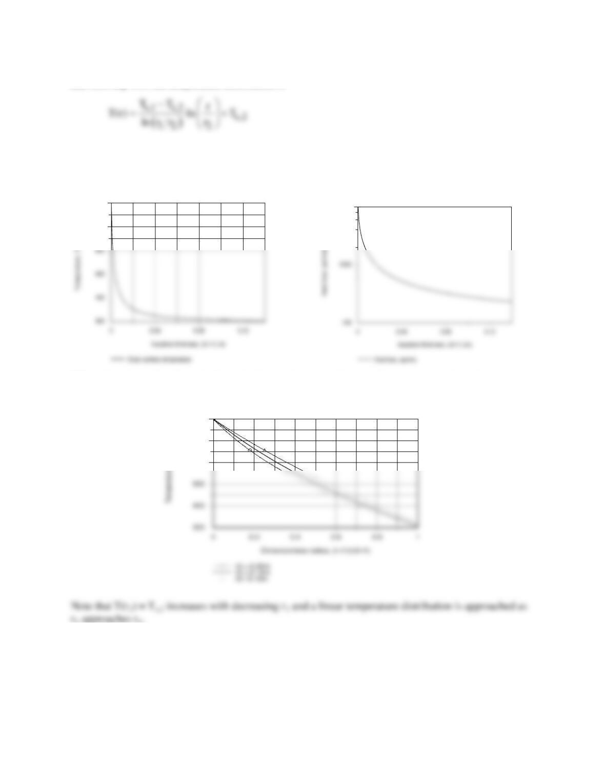
As shown below, the outer surface temperature of the insulation Ts,2 and the heat loss
q′
decay
precipitously with increasing insulation thickness from values of Ts,2 = Ts,1 = 800 K and
q′
= 11,600
W/m, respectively, at r2 = r1 (no insulation).
700
800
10000
When plotted as a function of a dimensionless radius, (r – r1)/(r2 – r1), the temperature decay becomes
more pronounced with increasing r2.
600
700
800
COMMENTS: An insulation layer thickness of 20 mm is sufficient to maintain the outer surface
temperature and heat rate below 350 K and 1000 W/m, respectively.
PROBLEM 3.40
KNOWN: Dimensions of components of a pipe-in–pipe device. Thermal conductivity of materials,
inner and outer heat transfer coefficients, outer fluid temperature.
FIND: (a) Maximum crude oil temperature to not exceed allowable service temperature of
polyurethane. (b) Maximum crude oil temperature to not exceed allowable service temperature of
polyurethane after insertion of aerogel layer.
SCHEMATIC:
ASSUMPTIONS: (1) Steady–state, one-dimensional conditions, (2) Negligible contact resistances,
(3) Constant properties.
PROPERTIES: Given, Steel: k = 35 W/m⋅K; polyurethane: k = 0.075 W/m⋅K; aerogel: k = 0.012
W/m⋅K.
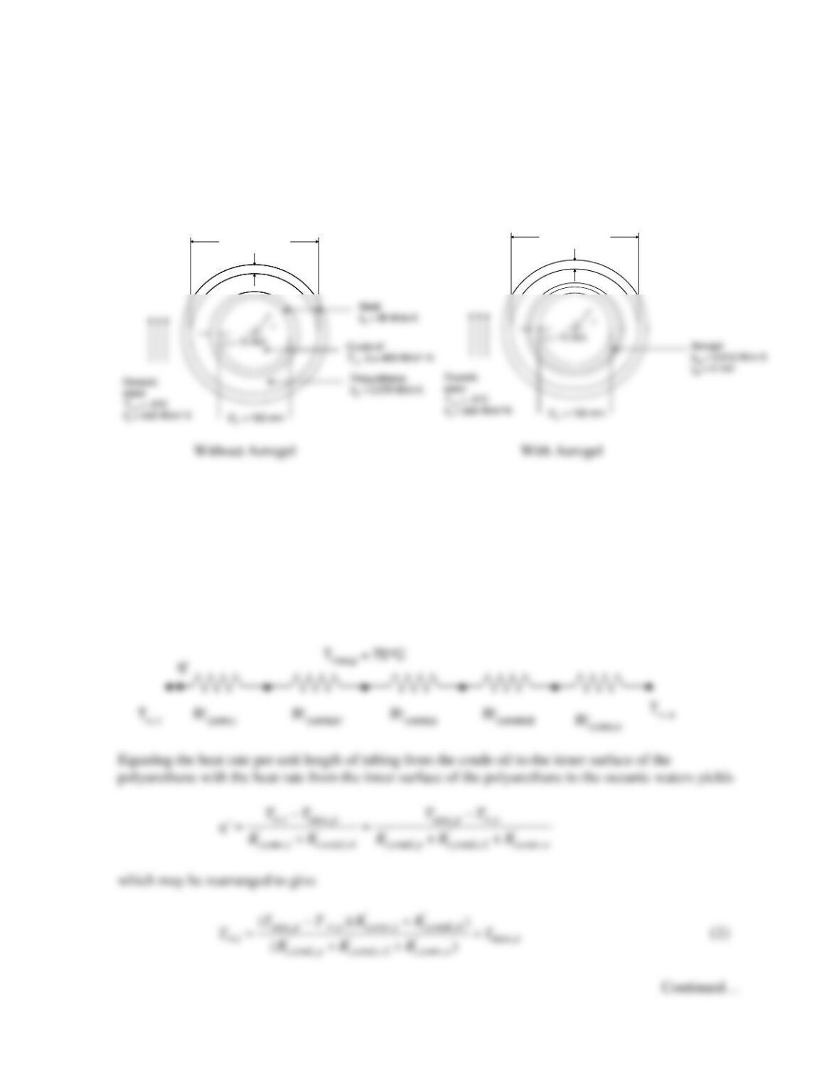
ANALYSIS: (a) The thermal resistance network for the case without the aerogel is shown below.
The maximum polyurethane temperature occus at its inner surface.
to= ti
Di,2 = 250 mm
to= ti
Di,2 = 250 mm
t
o
= t
i
D
i,2
= 250 mm
t
o
= t
i
D
i,2
= 250 mm
t
o
= t
i
D
i,2
= 250 mm
PROBLEM 3.40 (Cont.)
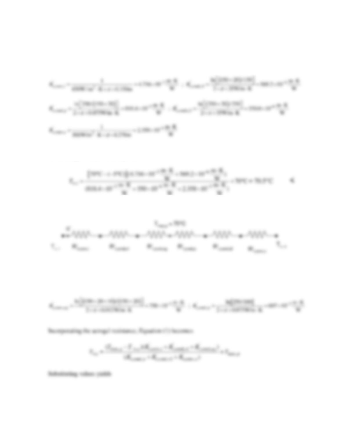
The various thermal resistances are evaluated as follows.
Substituting into Equation (1) yields
(b) The thermal resistance network for the case with the aerogel is shown below.
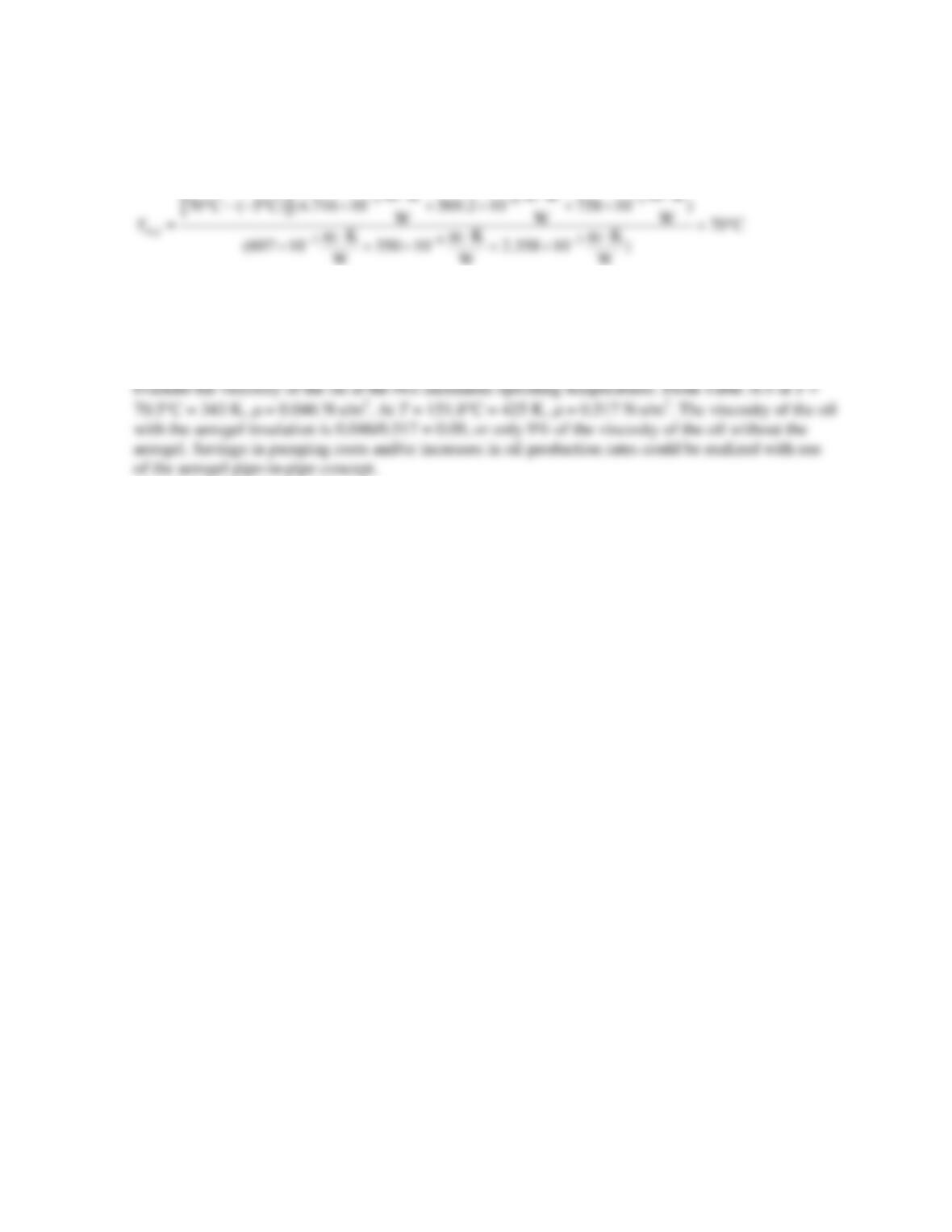
The thermal resistance values are as before, except the conduction resistance per unit length in the
polyurethane is decreased, since its thickness is reduced relative to part (a). In addition, the conduction
resistance for the aerogel must be evaluated. These two resistances are:
Continued…
PROBLEM 3.40 (Cont.)
= 151.8°C <
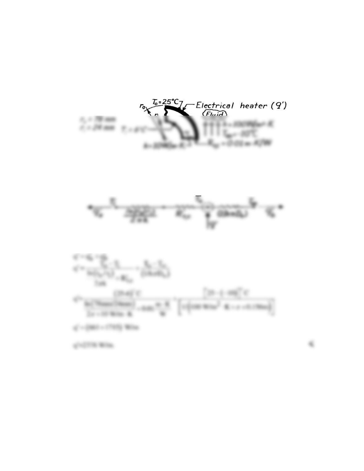
COMMENTS: Assuming the dynamic viscosity of crude oil is similar to that of engine oil, we may
PROBLEM 3.41
KNOWN: Inner and outer radii of a tube wall which is heated electrically at its outer surface
and is exposed to a fluid of prescribed h and T∞. Thermal contact resistance between heater
and tube wall and wall inner surface temperature.
FIND: Heater power per unit length required to maintain a heater temperature of 25°C.
SCHEMATIC:
ASSUMPTIONS: (1) Steady-state conditions, (2) One-dimensional conduction, (3) Constant
properties, (4) Negligible temperature drop across heater.
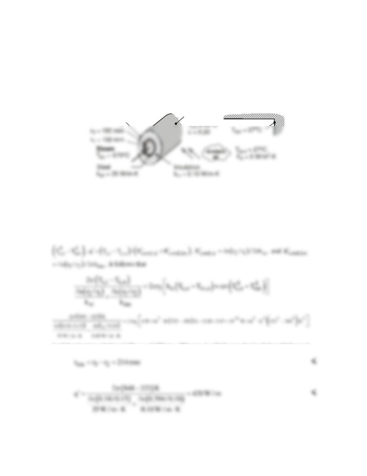
ANALYSIS: The thermal circuit has the form
Applying an energy balance to a control surface about the heater,
COMMENTS: The conduction, contact and convection resistances are 0.0188, 0.01 and 0.02
m ⋅K/W, respectively,
PROBLEM 3.42
KNOWN: Diameter, wall thickness and thermal conductivity of steel tubes. Temperature of steam
flowing through the tubes. Thermal conductivity of insulation and emissivity of aluminum sheath.
Temperature of ambient air and surroundings. Convection coefficient at outer surface and maximum
allowable surface temperature.
FIND: (a) Minimum required insulation thickness (r3 – r2) and corresponding heat loss per unit
length, (b) Effect of insulation thickness on outer surface temperature and heat loss.
SCHEMATIC:
Aluminum
r
3
o
ASSUMPTIONS: (1) Steady-state, (2) One-dimensional radial conduction, (3) Negligible contact
resistances at the material interfaces, (4) Negligible steam side convection resistance (T∞,i = Ts,i), (5)
Negligible conduction resistance for aluminum sheath, (6) Constant properties, (7) Large
surroundings.
ANALYSIS: (a) To determine the insulation thickness, an energy balance must be performed at the
outer surface, where
conv,o rad
qq q.
′′ ′
= +
With
( )
conv,o 3 o s,o ,o
q 2 rh T T ,
π
∞
′= −
rad 3
q 2r
π
′=
eσ
A trial–and-error solution yields r3 = 0.394 m = 394 mm, in which case the insulation thickness is
The heat rate is then
(b) The effects of r3 on Ts,o and
q′
have been computed and are shown below.
Continued …