PROBLEM 3.121
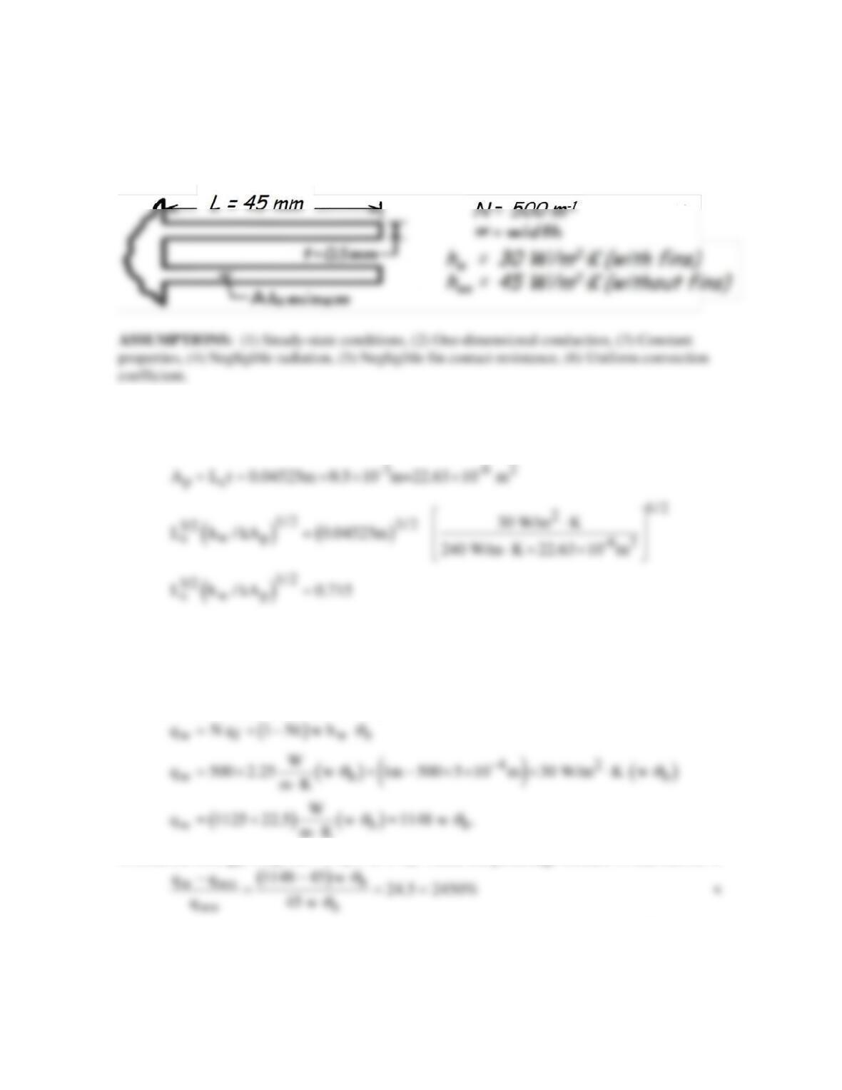
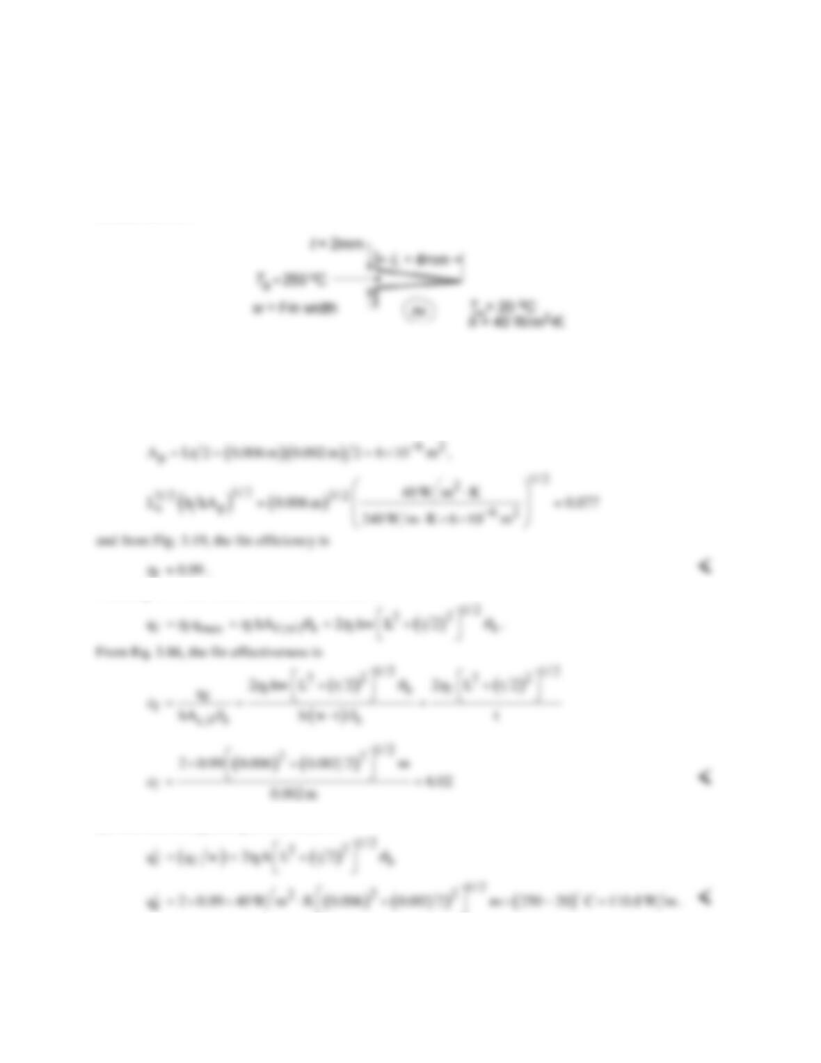
KNOWN: Dimensions and number of rectangular aluminum fins. Convection coefficient with and
without fins.
FIND: Percentage increase in heat transfer resulting from use of fins.
SCHEMATIC:
PROPERTIES: Table A-1, Aluminum, pure: k ≈ 240 W/m⋅K.
ANALYSIS: Evaluate the fin parameters
c
L L+t/2 0.04525m= =
It follows from Fig. 3.19 that ηf ≈ 0.75. Hence,
f f max w b
q q 0.75 h 2wL
ηθ
= =
( ) ( )
2
f bb
q 0.75 30 W/m K 2 0.05m w 2.25 W/m K w
θθ
= × ⋅ ×× × = ⋅
With the fins, the heat transfer from the walls is
Without the fins, qwo = hwo 1m × w θb = 45 w θb. Hence the percentage increase in heat transfer is
COMMENTS: If the infinite fin approximation is made, it follows that qf = (hPkAc)1/2 θb
=[hw2wkwt]1/2 θb = (30 × 2 × 240 × 5×10-4)1/2 w θb = 2.68 w θb. Hence, qf is overestimated with use
of the infinite fin assumption.
PROBLEM 3.122
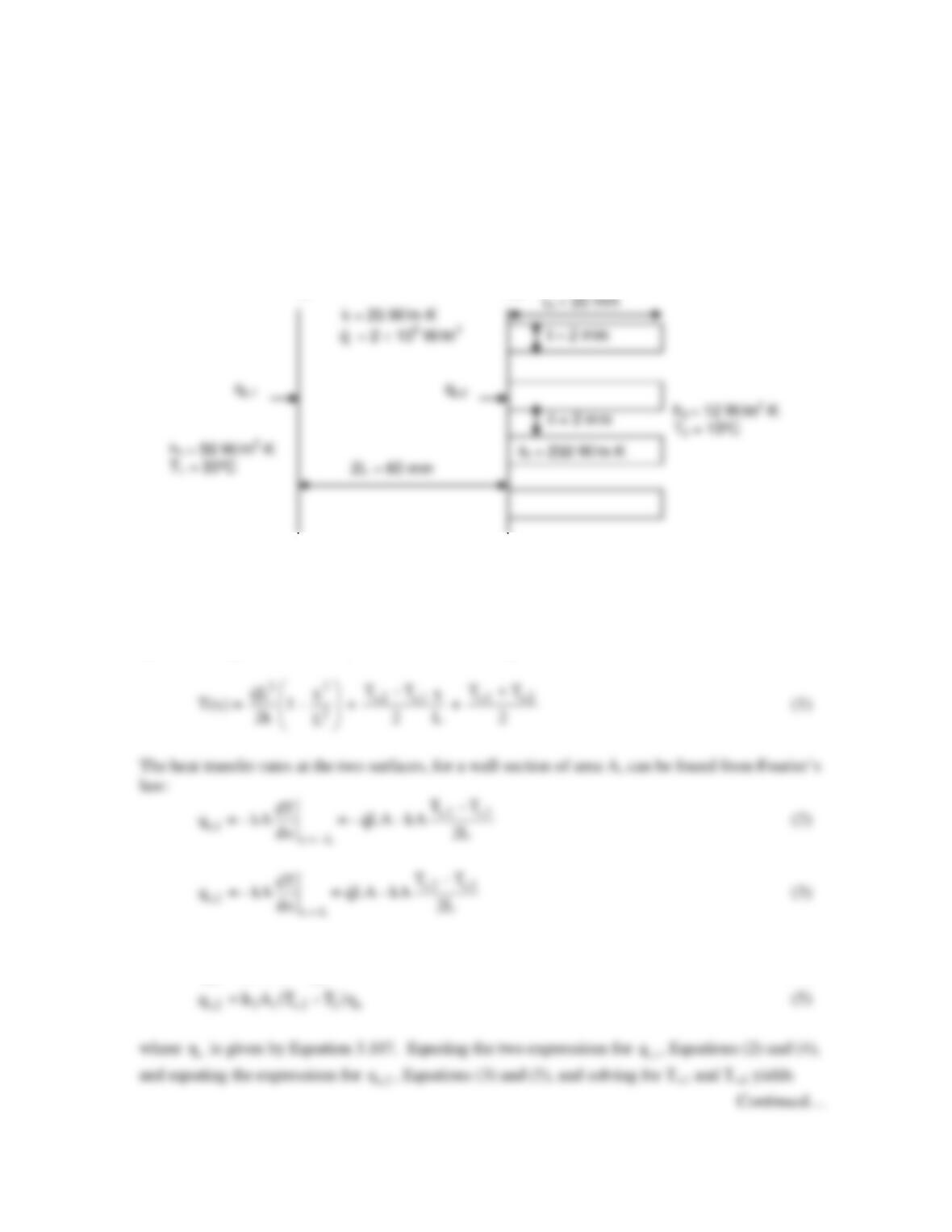
KNOWN: Wall with known heat generation rate, thermal conductivity, and thickness.
Dimensions and thermal conductivity of fins. Heat transfer coefficients and environment
temperatures.
FIND: Maximum temperature.
SCHEMATIC:
ASSUMPTIONS: (1) Steady–state conditions, (2) Wall surface temperatures are uniform. (3) No
contact resistance between fins and wall, (4) Heat transfer from the fin tips can be neglected.
ANALYSIS: The temperature distribution in a wall with uniform volumetric heat generation and
specified temperature boundary conditions is, from Equation 3.46
We can express these same heat transfer rates alternatively, as follows:
s,1 1 1 s,1
q = h A(T – T )
(4)
q
L
q
T
s,1
T
s,2
PROBLEM 3.122 (Cont.)
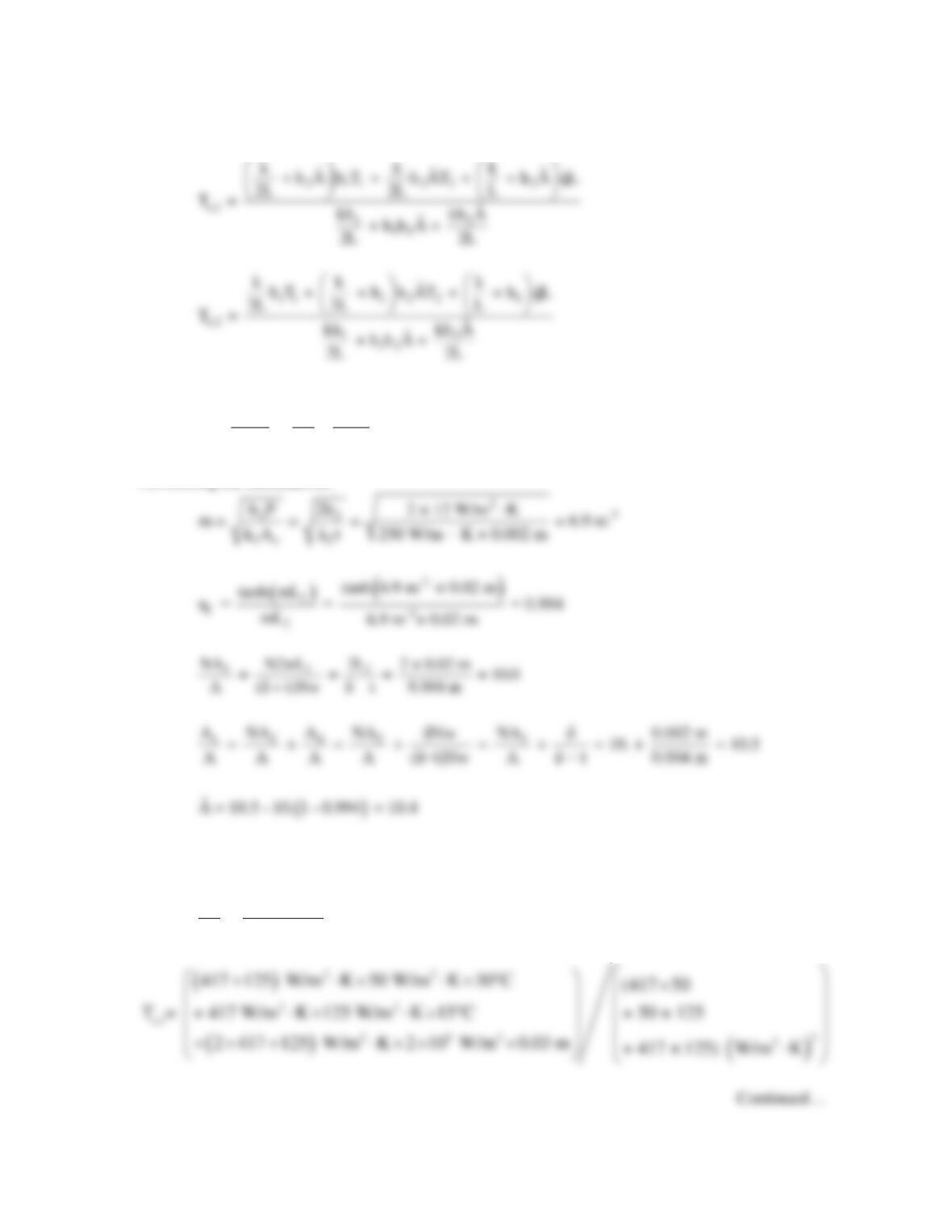
where
( )
to t ff
AηA
NA
A = = – 1 – η
A AA
Performing the calculations:
22
2
h A = 12 W/m K × 10.4 = 125 W/m K⋅⋅
2
k 25 W/m K
= = 417 W/m K
2L 0.06 m
⋅⋅
Thus
PROBLEM 3.122 (Cont.)
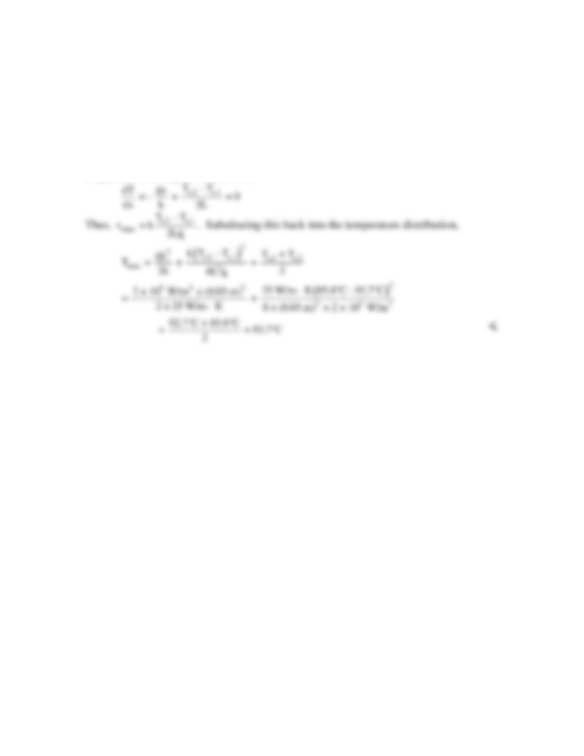
Ts,1 = 92.7ºC
Similarly,
Ts,2 = 85.8ºC
The location of the maximum temperature in the wall can be found by setting the gradient of the
temperature (from Equation (1)) to zero:
PROBLEM 3.123
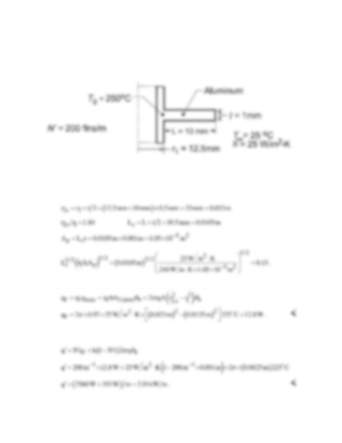
KNOWN: Dimensions, base temperature and environmental conditions associated with a triangular,
aluminum fin.
FIND: (a) Fin efficiency and effectiveness, (b) Heat dissipation per unit width.
SCHEMATIC:
ASSUMPTIONS: (1) Steady-state conditions, (2) One-dimensional conduction, (3) Constant properties,
(4) Negligible radiation and base contact resistance, (5) Uniform convection coefficient.
PROPERTIES: Table A-1, Aluminum, pure (T ≈ 400 K): k = 240 W/m⋅K.
ANALYSIS: (a) With Lc = L = 0.006 m, find
f0.99
From Eq. 3.91 and Table 3.5, the fin heat rate is
(b) The heat dissipation per unit width is
COMMENTS: The parabolic profile is known to provide the maximum heat dissipation per unit fin
mass.
PROBLEM 3.124
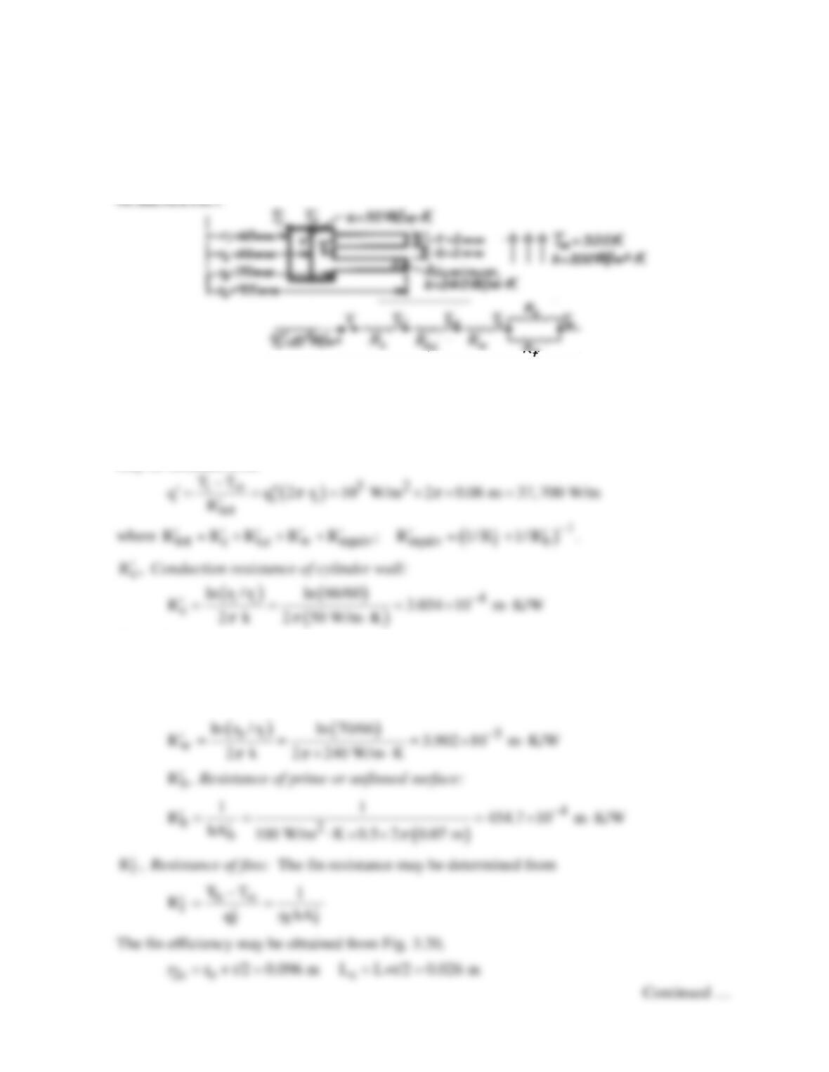
KNOWN: Dimensions and base temperature of an annular, aluminum fin of rectangular profile.
Ambient air conditions.
FIND: (a) Fin heat loss, (b) Heat loss per unit length of tube with 200 fins spaced at 5 mm increments.
SCHEMATIC:
ASSUMPTIONS: (1) Steady-state conditions, (2) One-dimensional conduction, (3) Constant properties,
(4) Negligible radiation and contact resistance, (5) Uniform convection coefficient.
PROPERTIES: Table A-1, Aluminum, pure (T ≈ 400 K): k = 240 W/m⋅K.
ANALYSIS: (a) The fin parameters for use with Figure 3.20 are
Hence, the fin effectiveness is ηf ≈ 0.97, and from Eq. 3.91 and Fig. 3.6, the fin heat rate is
(b) Recognizing that there are N = 200 fins per meter length of the tube, the total heat rate considering
contributions due to the fin and base (unfinned) surfaces is
COMMENTS: Note that, while covering only 20% of the tube surface area, the tubes account for more
than 85% of the total heat dissipation.
PROBLEM 3.125
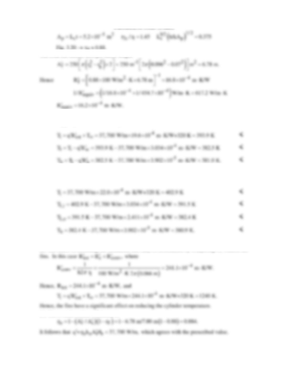
KNOWN: Dimensions and materials of a finned (annular) cylinder wall. Heat flux and
ambient air conditions. Contact resistance.
FIND: Surface and interface temperatures (a) without and (b) with an interface contact
resistance.
ASSUMPTIONS: (1) One-dimensional, steady-state conditions, (2) Constant properties, (3)
Uniform h over surfaces, (4) Negligible radiation.
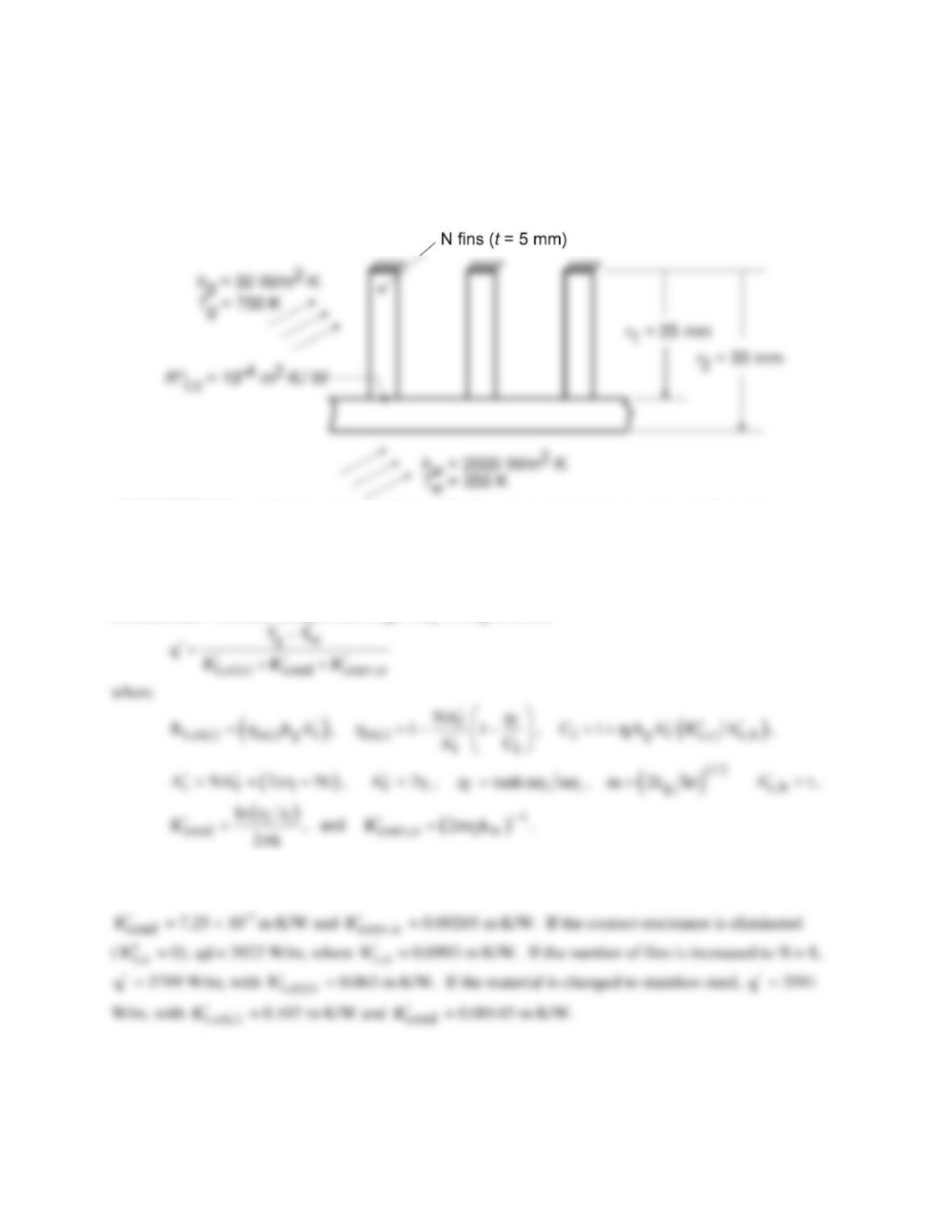
ANALYSIS: The analysis may be performed per unit length of cylinder or for a 4 mm long
section. The following calculations are based on a unit length. The inner surface temperature
may be obtained from
′
Rt,c,
Contact resistance:
42 4
t,c t,c 1
R R / 2 r 10 m K/W/2 0.066 m 2.411 10 m K/W
ππ
—
′ ′′
= = ⋅ × =×⋅
w
R,
′
Conduction resistance of aluminum base:
PROBLEM 3.125 (Cont.)
The total fin surface area per meter length
Neglecting the contact resistance,
( )
44
tot
R 3.034 0.390 16.2 10 m K/W 19.6 10 m K/W
—
′= + + ⋅=× ⋅
b1 b
Including the contact resistance,
()
44 4
tot
R 19.6 10 2.411 10 m K/W 22.0 10 m K/W
— –
′=×+ × ⋅=× ⋅
COMMENTS: (1) The effect of the contact resistance is small.
(2) The effect of including the aluminum fins may be determined by computing Ti without the
(3) The overall surface efficiency is
PROBLEM 3.126
KNOWN: Internal and external convection conditions for an internally finned tube. Fin/tube
dimensions and contact resistance.
FIND: Heat rate per unit tube length and corresponding effects of the contact resistance, number of fins,
and fin/tube material.
SCHEMATIC:
ASSUMPTIONS: (1) Steady-state conditions, (2) One-dimensional heat transfer, (3) Constant
properties, (4) Negligible radiation, (5) Uniform convection coefficient on finned surfaces, (6) Tube wall
may be unfolded and approximated as a plane surface with N straight rectangular fins.
PROPERTIES: Copper: k = 400 W/m⋅K; St.St.: k = 20 W/m⋅K.
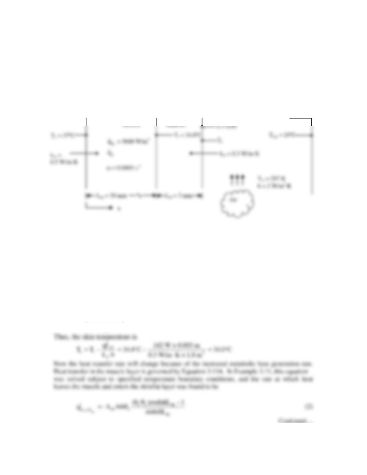
ANALYSIS: The heat rate per unit length may be expressed as
Using the IHT Performance Calculation, Extended Surface Model for the Straight Fin Array, the
following results were obtained. For the base case,
q′
= 3857 W/m, where
t,o(c)
R′
= 0.101 m⋅K/W,
¢
t,o(c)
COMMENTS: The small reduction in
¢
q
associated with use of stainless steel is perhaps surprising, in
view of the large reduction in k. However, because
g
h
is small, the reduction in k does not significantly
reduce the fin efficiency (
f
η
changes from 0.994 to 0.891). Hence, the heat rate remains large. The
influence of k would become more pronounced with increasing
g
h
.
PROBLEM 3.127
KNOWN: Dimensions and thermal conductivities of a muscle layer and a skin/fat layer. Skin
emissivity and surface area. Metabolic heat generation rate and perfusion rate within the muscle
layer. Core body and arterial temperatures. Blood density and specific heat. Ambient conditions.
FIND: Perspiration rate to maintain same skin temperature as in Example 3.11.
SCHEMATIC:
ASSUMPTIONS: (1) Steady–state conditions, (2) One–dimensional heat transfer through the
muscle and skin/fat layers, (3) Metabolic heat generation rate, perfusion rate, arterial temperature,
blood properties, and thermal conductivities are all uniform, (4) Radiation heat transfer
coefficient is known from Example 1.7, (5) Solar radiation is negligible, (6) Conditions are the
same everywhere on the torso, limbs, etc., (7) Perspiration on skin has a negligible effect on heat
transfer from the skin to the environment, that is, it adds a negligible thermal resistance and
doesn’t change the emissivity.
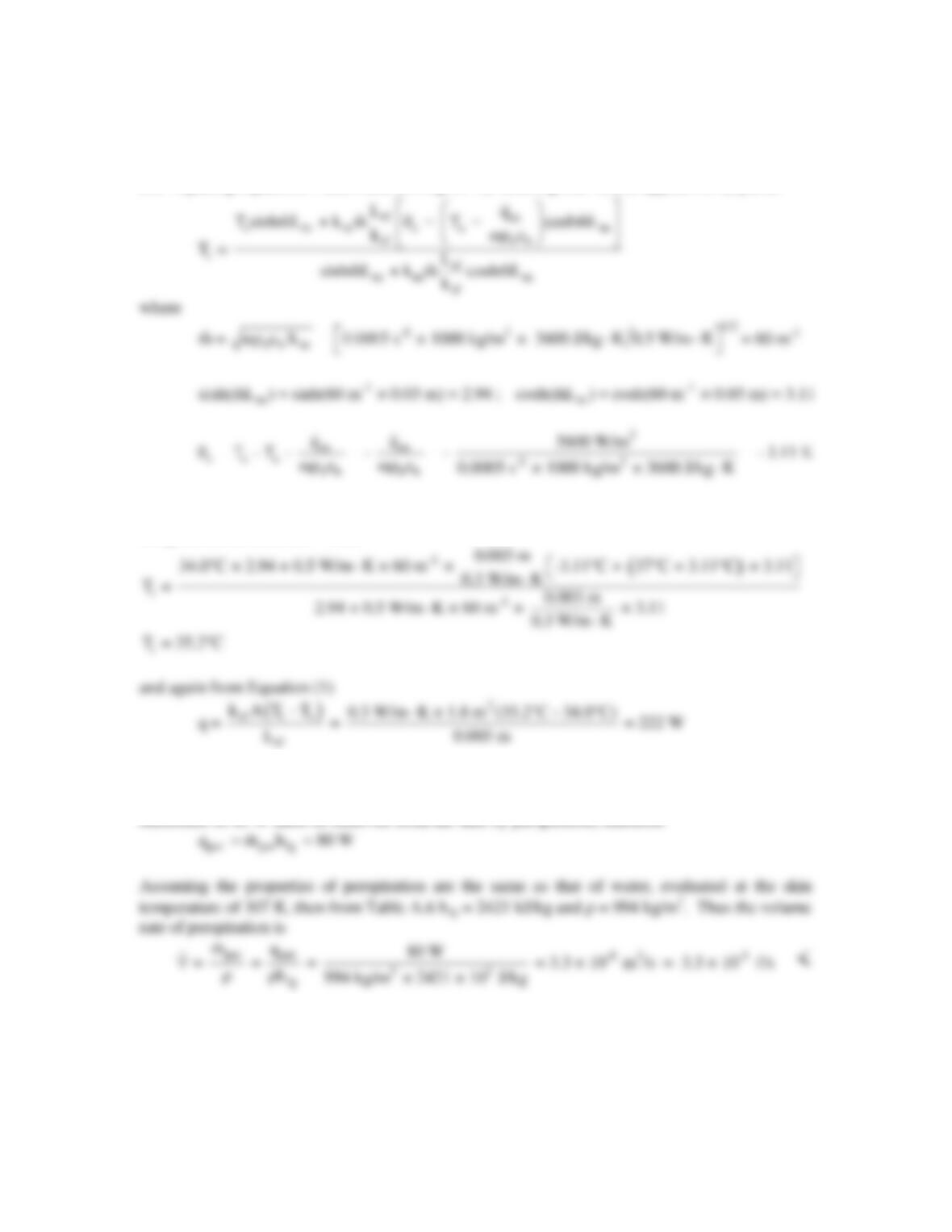
ANALYSIS: First we need to find the skin temperature, Ts, for the conditions of Example 3.11,
in the air environment. Both q and Ti, the interface temperature between the muscle and the
skin/fat layer, are known. The rate of heat transfer across the skin/fat layer is given by
( )
sf i s
sf
k AT T
qL
–
=
(1)
Continued…
PROBLEM 3.127 (Cont.)
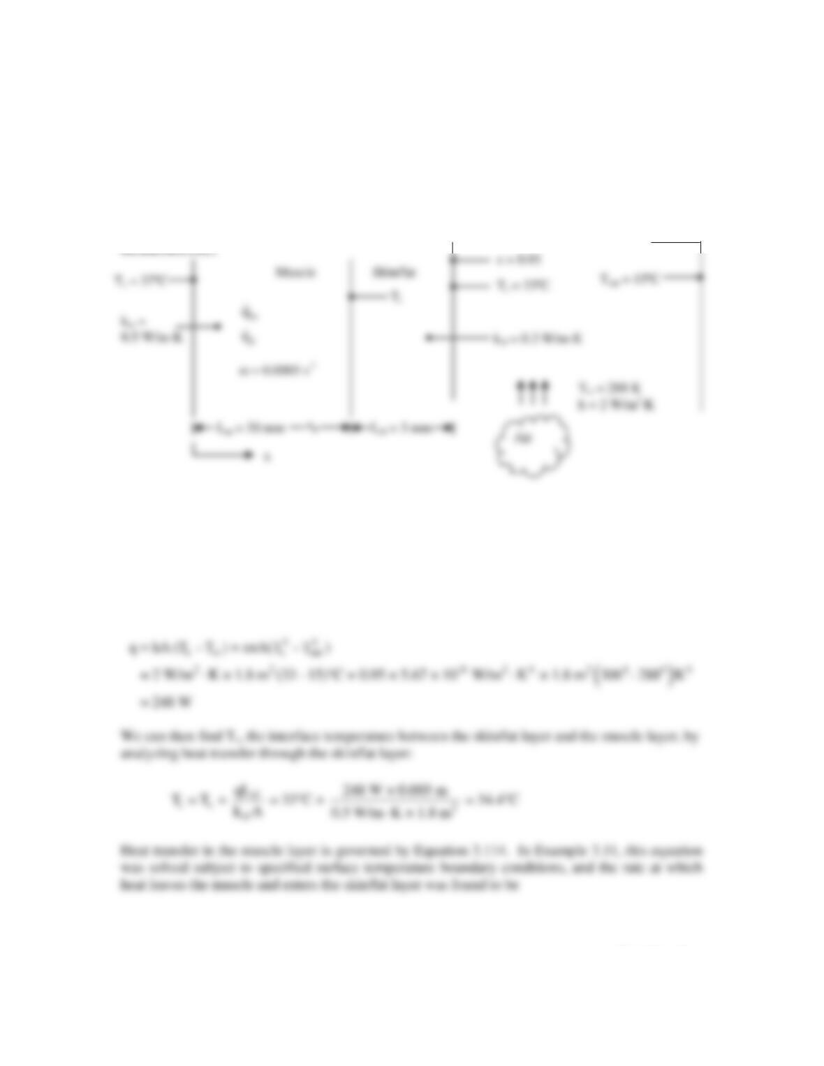
This must equal the rate at which heat is transferred across the skin/fat layer, given by Equation
(1). Equating Equations 1 and 2 and solving for Ti, recalling that Ti also appears in θi, yields
The excess temperature can be expressed in kelvins or degrees Celsius, since it is a
temperature difference. Thus
Since the skin temperature is unchanged from Example 3.11, the rate of heat transfer to the
environment by convection and radiation will remain the same, and is therefore still 142 W. The
difference of 80 W must be removed from the skin by perspiration, therefore
COMMENTS: (1) This is a moderate rate of perspiration. In one hour, it would account for
around 0.1
. (2) In reality, our bodies adjust in many ways to maintain core and skin
temperatures. Exercise will likely cause an increase in perfusion rate near the skin surface, to
locally elevate the temperature and increase the rate of heat transfer to the environment.
PROBLEM 3.128
KNOWN: Dimensions and thermal conductivities of a muscle layer and a skin/fat layer. Skin
emissivity and surface area. Skin temperature. Perfusion rate within the muscle layer. Core
body and arterial temperatures. Blood density and specific heat. Ambient conditions.
FIND: Metabolic heat generation rate to maintain skin temperature at 33ºC.
ASSUMPTIONS: (1) Steady–state conditions, (2) One-dimensional heat transfer through the
muscle and skin/fat layers, (3) Metabolic heat generation rate, perfusion rate, arterial temperature,
blood properties, and thermal conductivities are all uniform, (4) Solar radiation is negligible, (5)
Conditions are the same everywhere on the torso, limbs, etc.
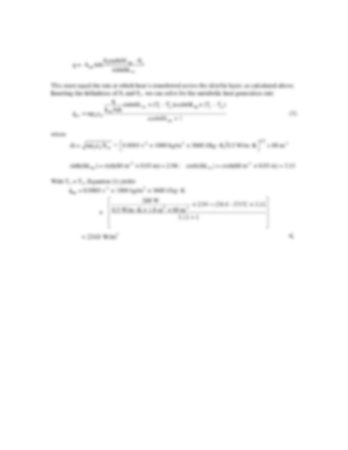
ANALYSIS: Since we know the skin temperature and environment temperature, we can find the
heat loss rate from the skin surface to the environment:
Continued…
PROBLEM 3.128 (Cont.)
COMMENT: (1) Shivering can increase the metabolic heat generation rate by up to five to six
times the resting metabolic rate. The value found here is approximately three times the metabolic
heat generation rate given in Example 3.11, so it is well within what can be produced by
shivering. (2) In the water environment, even with the original 24ºC water temperature, shivering
would be insufficient to maintain a comfortable skin temperature.
PROBLEM 3.129
KNOWN: Dimensions and thermal conductivities of a muscle layer and a skin/fat layer.
Metabolic heat generation rate and perfusion rate within the muscle layer. Arterial temperature.
Blood density and specific heat. Ambient conditions.
FIND: Heat loss rate from body and temperature at inner surface of the skin/fat layer.
SCHEMATIC:
ASSUMPTIONS: (1) Steady–state conditions, (2) One-dimensional heat transfer through the
muscle and skin/fat layers, (3) Metabolic heat generation rate, perfusion rate, arterial temperature,
blood properties, and thermal conductivities are all uniform, (4) Radiation heat transfer
coefficient is known from Example 1.5.
ANALYSIS:
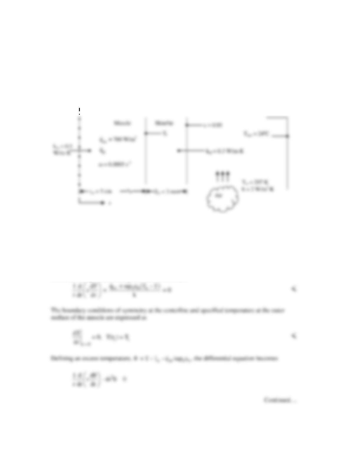
(a) Conduction with heat generation is expressed in radial coordinates by Equation 3.54. With
metabolic heat generation and perfusion, this becomes
PROBLEM 3.129 (Cont.)
where
2
bb
m = ωρ c /k
. The general solution to the differential equation is given in Section 3.6.4
Solving for c1 we now have the complete solution for θ:
0
i
01
I (mr)
θ = θ I (mr )
(1) <
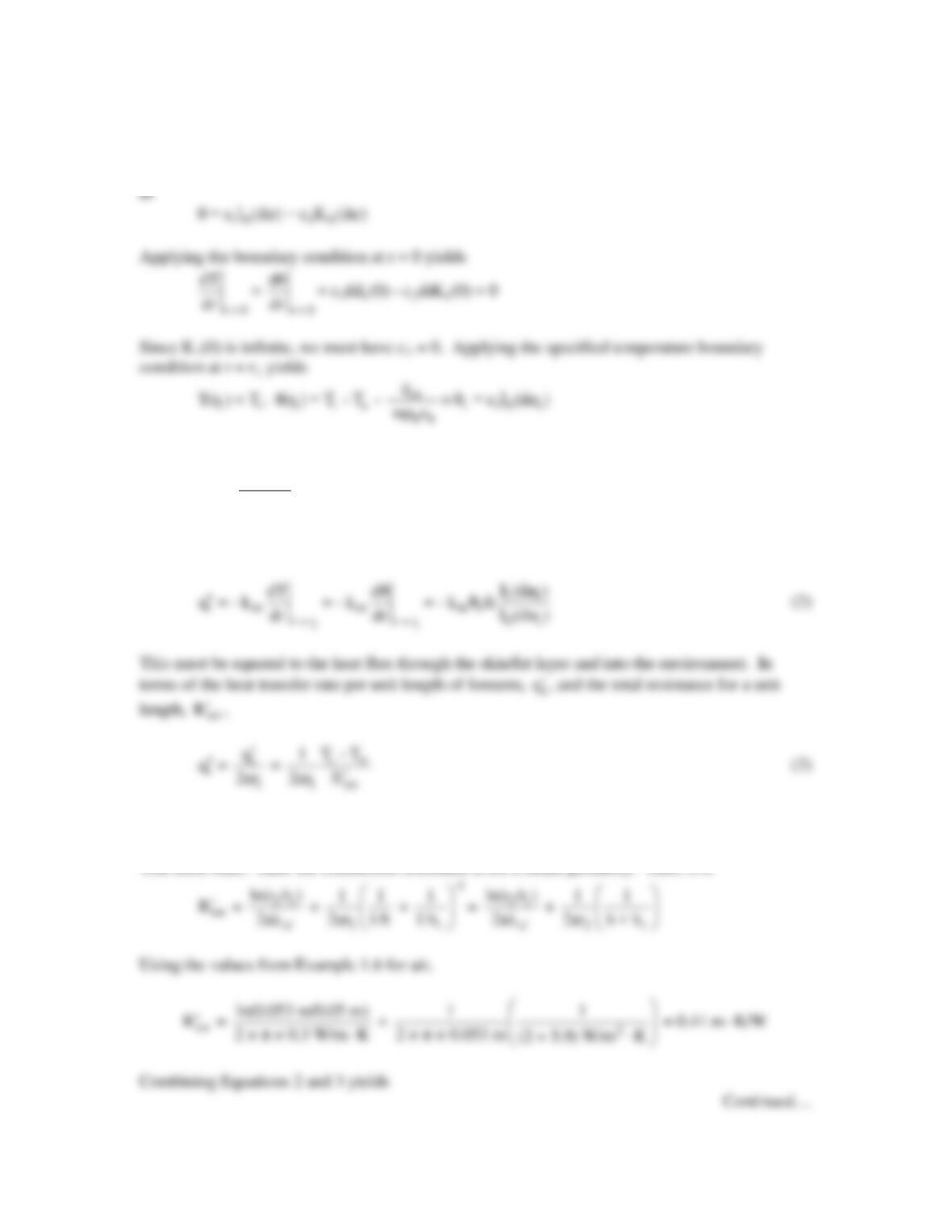
(b) The heat flux at the outer surface of the muscle is given by
As in Example 3.1 and for exposure of the skin to the air,
tot
R′
accounts for conduction through
the skin/fat layer in series with heat transfer by convection and radiation, which act in parallel
with each other. Here the conduction resistance is for a radial geometry. Thus, it is
PROBLEM 3.129 (Cont.)
where
and from Table B.5
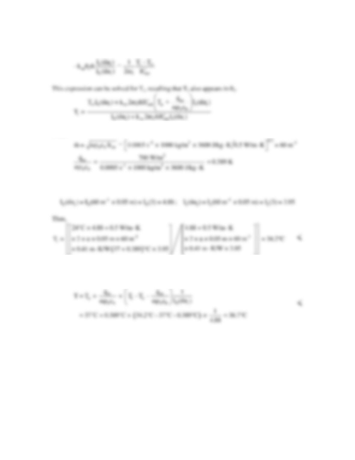
(c) The maximum temperature occurs at the centerline of the forearm, r = 0, thus from Equation
1, with I0(0) = 1,
COMMENTS: (1) The maximum temperature is very close to the core body temperature
of 37ºC, as would be expected. (2) Pennes [17] conducted an experimental investigation
of the temperature distribution in human forearms, by inserting thermocouples into living
subjects.
PROBLEM 3.130
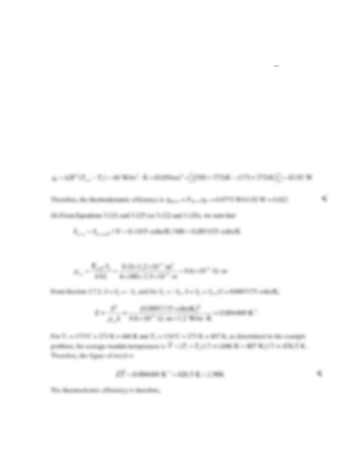
KNOWN: Thermoelectric module properties and performance, as given in Example 3.12.
FIND: (a) The thermodynamic efficiency,
η
therm ≡ PM=1/q1, (b) the figure of merit
ZT
for one module,
and the thermoelectric efficiency,
η
TE. (c) the Carnot efficiency,
η
Carnot = 1 – T2/T1, (d) the value of
η
TE
based upon the inappropriate use of T∞,1 and T∞,2 (e) the thermoelectric efficiency based upon the correct
usage of T1 and T2 in Equation 3.128, and the Carnot efficiency for the case where h1 = h2 → ∞.
ASSUMPTIONS: (1) Steady–state, one–dimensional conduction, (2) Negligible contact resistances, (3)
Negligible radiation exchange and gas phase conduction inside the module, (4) Negligible conduction
resistance due to metallic contacts and ceramic insulators, (5) The properties of the two semiconductors
are identical and Sp = – Sn.
ANALYSIS: (a) From Example 3.12 the electrical power per module is PM = 1 = Ptot/M = 46.9 W/48 =
0.9773 W. The heat input to one module may be evaluated from Equation 3 of the solution to the example
problem as
and
Continued…
PROBLEM 3.130 (Cont.)
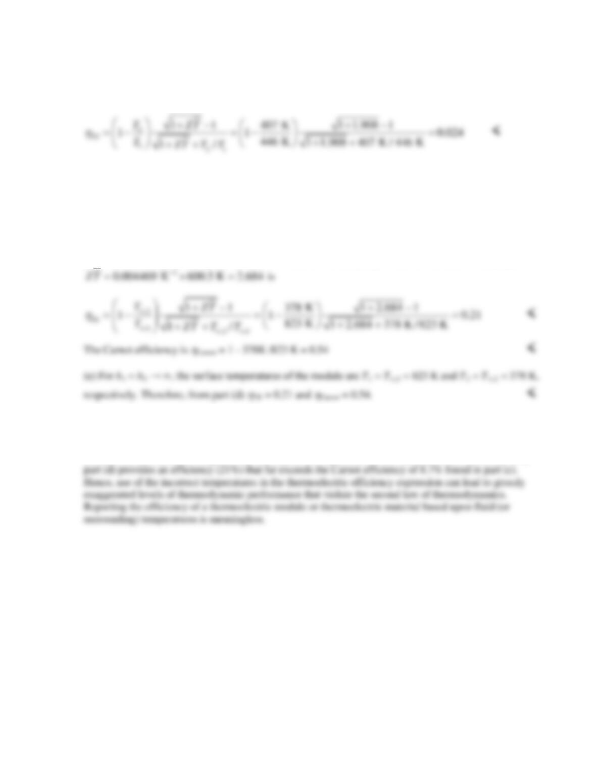
We note that the thermodynamic efficiency is less than the thermoelectric efficiency based on the figure of
merit and the surface temperatures of the module. The thermoelectric efficiency is the maximum possible
efficiency for the case when the load resistance is optimized.
(c) The Carnot efficiency is
η
Carnot = 1 – 407K /446 K = 0.087 <
(d) The value of
η
TE based upon T∞,1 = 550°C + 273 K = 823 K, T∞,2 = 105°C + 273 K = 378 K, and
COMMENTS: (1) The conversion efficiency for the thermoelectric modules of Example 3.12 is quite
small, approximately 2%. (2) The conversion efficiency can be increased by an order of magnitude (to
21%) by utilizing thermal management approaches that will increase the temperature difference across the
module. (c) The incorrect usage of T∞,1 and T∞,2 in the expression for the thermoelectric efficiency as in
PROBLEM 3.131
KNOWN: Dimensions of thermoelectric module and heat sinks. Convection conditions, heat sink
thermal conductivity, thermoelectric module performance parameters, load electrical resistance.
Contact resistance between thermoelectric module and heat sinks.
FIND: (a) Sketch of the equivalent thermal circuit and electrical power generated without the heat
sinks. (b) Sketch of the equivalent thermal circuit and electrical power generated with the heat sinks.
SCHEMATIC:
ASSUMPTIONS: (1) Steady–state, one–dimensional conduction, (2) Constant properties, (3)
Negligible radiation, (4) Adiabatic fin tips for part (b), (5) Convection coefficients same in parts (a)
and (b) and the same on the sides of the fin arrays.
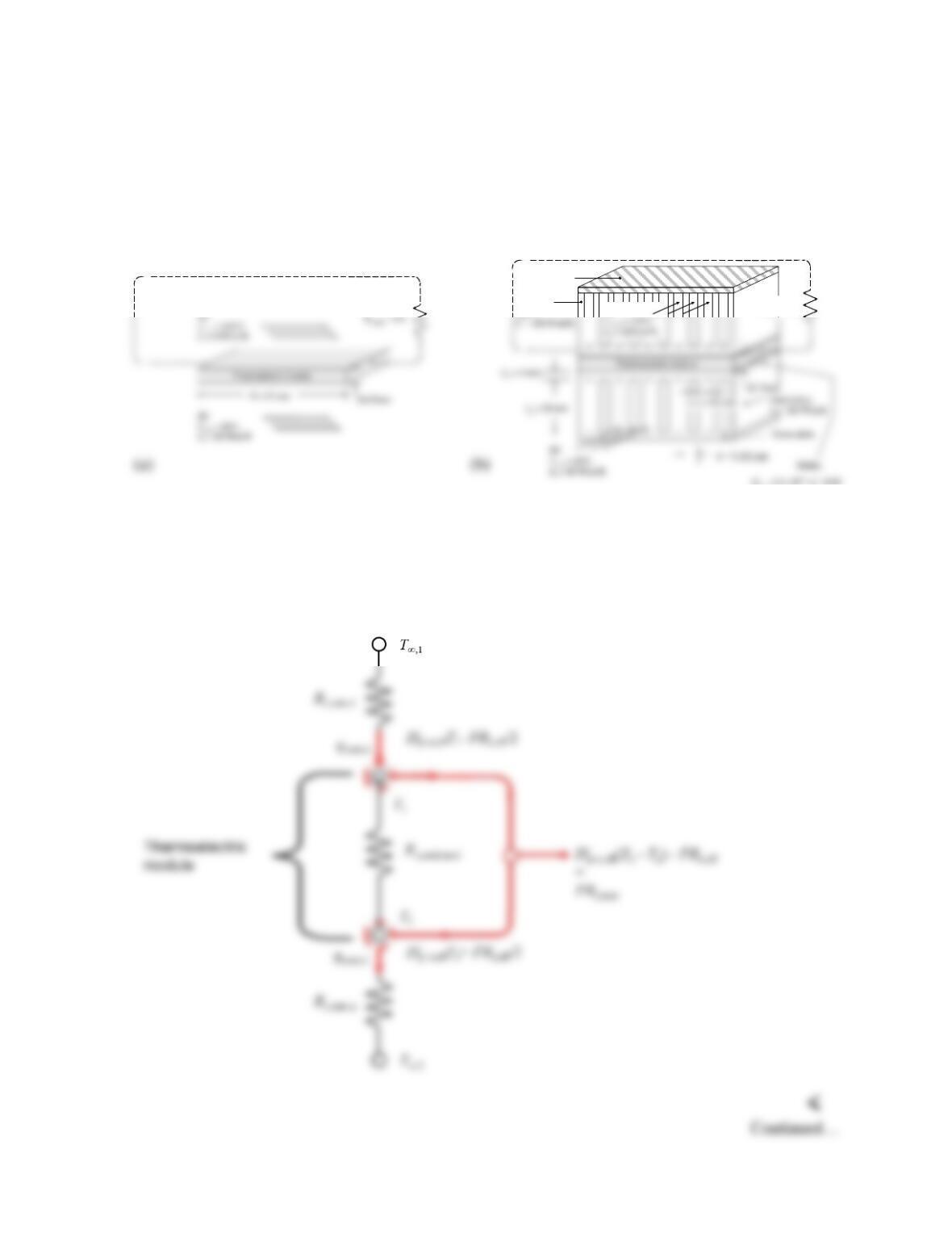
ANALYSIS: (a) Without the heat sinks, the equivalent thermal circuit is shown in Figure 3.24b as
replicated below.
R
e,load
= 4 Ω
Heat
sink 1
Air
,
2.5 10 m K/W
tc
R
=×⋅
Cover plate
R
e,load
= 4 Ω
Heat
sink 1
Air
,
2.5 10 m K/W
tc
R
=×⋅
Cover plate
PROBLEM 3.131 (Cont.)
The analysis can proceed as in Example 3.12. The conduction resistance of one module is the same as
in the example, namely
Newton’s law of cooling may be written at each surface as
The electric power produced by a single module, PN, is equal to the electric power dissipated in the load
resistance. Equating the expression for PN from Equation 3.127 to the electric power dissipated in the load
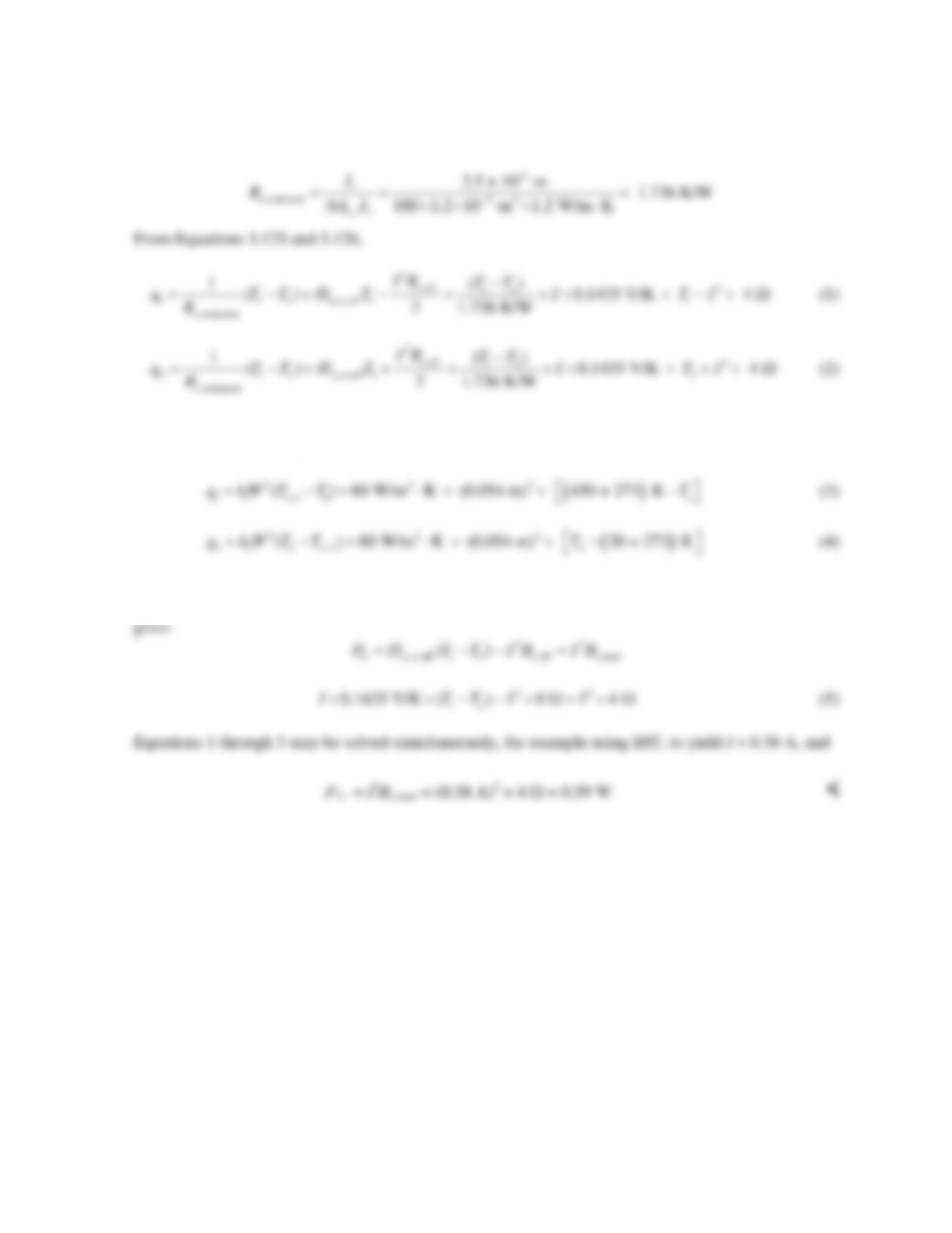
(b) The thermal circuit associated with the thermoelectric module is unchanged, but each convection
resistance must be replaced with the total thermal resistance, Rtot, associated with the contact
resistance, fin array base, and overall resistance of the fin array, as shown below. Also, qconv,1 and
qconv,2 have been replaced with the more general terms q1 and q2.
Continued…