9
CHAPTER 3
2. A time series consists of data that are collected, recorded, or observed over successive
increments of time.
3. The secular trend of a time series is the long-term component that represents the growth or
decline in the series over an extended period of time. The cyclical component is the wave-
5. The autocorrelation coefficient measures the correlation between a variable, lagged one or
more periods, and itself.
6. The correlogram is a useful graphical tool for displaying the autocorrelations for various
lags of a time series. Typically, the time lags are shown on a horizontal scale and the
7. a. nonstationary series
8. a. stationary series
b. random series
9. Naive methods, simple averaging methods, moving averages, and Box-Jenkins methods.
10
10. Moving averages, simple exponential smoothing, Holt’s linear exponential smoothing,
simple regression, growth curves, and Box-Jenkins methods. Examples are: sales
11. Classical decomposition, census II, Winters exponential smoothing, time series multiple
13. 1985 2,413 – 1999 2358 114
1986 2,407 -6 2000 2329 -29
1987 2,403 -4 2001 2345 16
1988 2,396 -7 2002 2254 -91
14. 0 1.96 ( 1
80 ) = 0 1.96 (.1118) = 0 .219
15. a. MPE
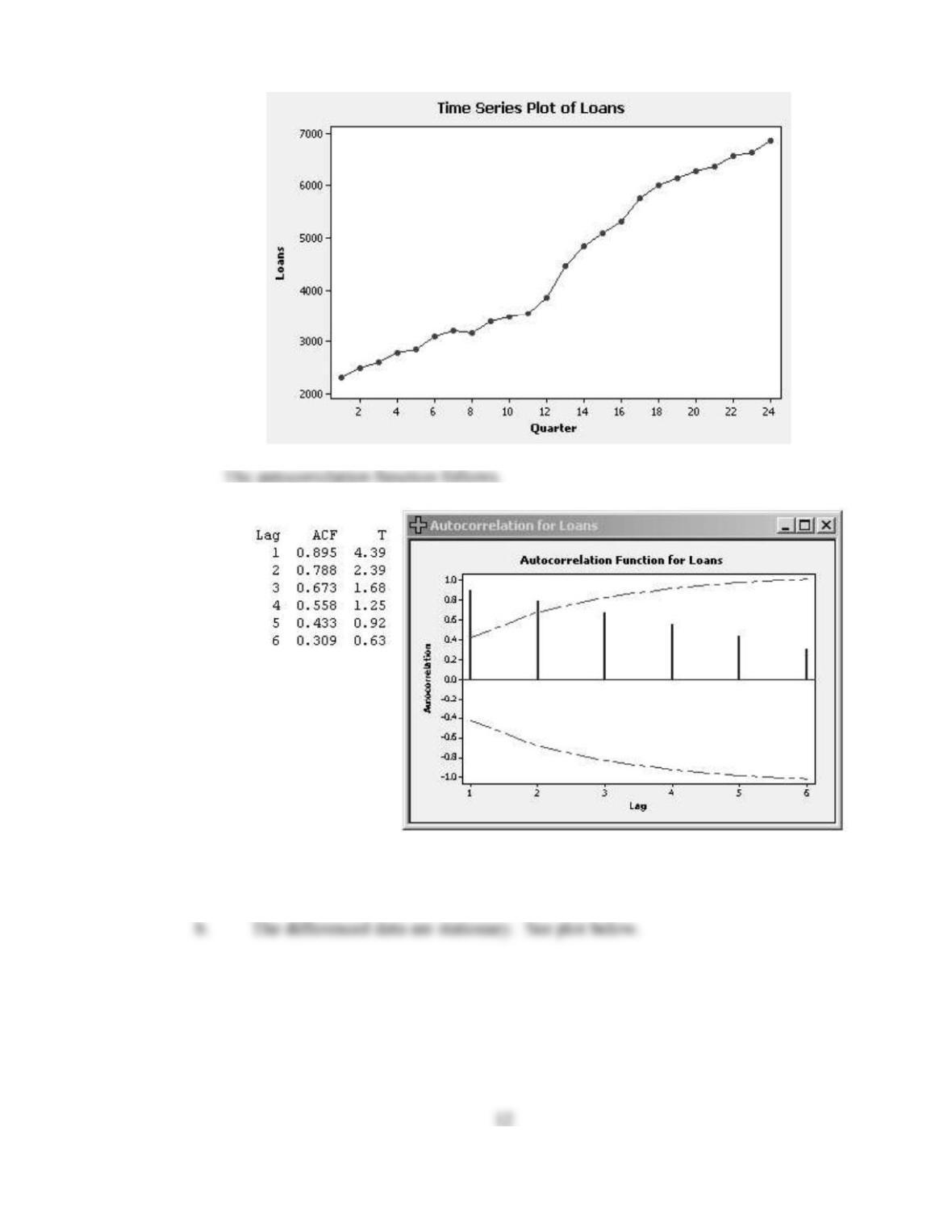
17. a. r1 = .895
H01 = 0 H11 0
k
r
11
r
t
=
0895. = 4.39
SE(
) = n
r
i
i
1
21
=24
895.21
1
i=2 6
.= .33
18. a. r1 = .376
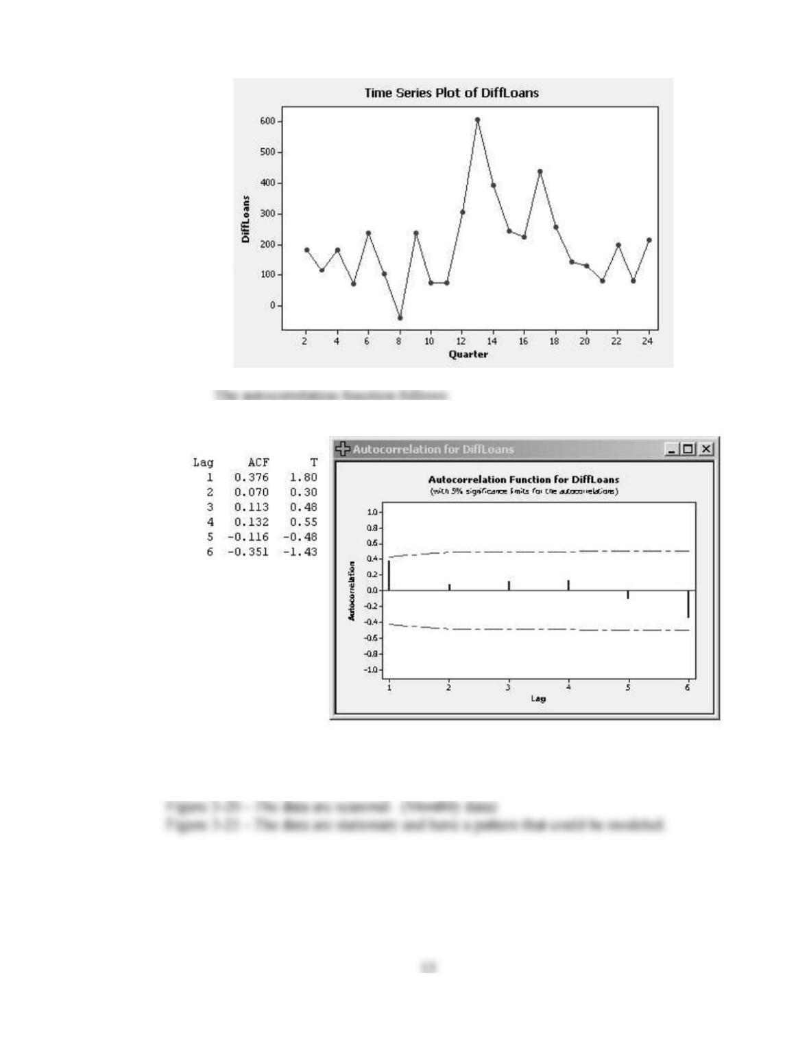
19. Figure 3-18 – The data are nonstationary. (Trending data)
Figure 3-19 – The data are random.
14
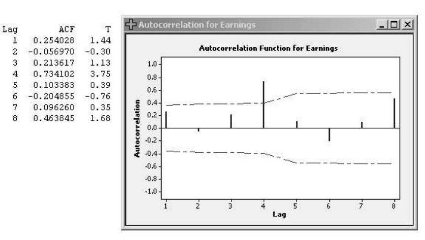
20.
The data have a quarterly seasonal pattern as shown by the significant autocorrelation
at time lag 4. First quarter earnings tend to be high, third quarter earnings tend to be low.
a. Time Data Forecast Error
6 .34 .47 -.13 .13 .0169 .3824 -.3824
7 .30 .34 -.04 .04 .0016 .1333 -.1333
8 .39 .30 .09 .09 .0081 .2308 .2308
9 .63 .39 .24 .24 .0576 .3810 .3810
10 .43 .63 -.20 .20 .0400 .4651 -.4651
21 .94 .63 .31 .31 .0961 .3298 .3298
22 .56 .94 -.38 .38 .1444 .6786 -.6786
23 .50 .56 -.06 .06 .0036 .1200 -.1200
24 .65 .50 .15 .15 .0225 .2308 .2308
25 .95 .65 .30 .30 .0900 .3158 .3158
5.85 1.6865 11.2227 -2.1988
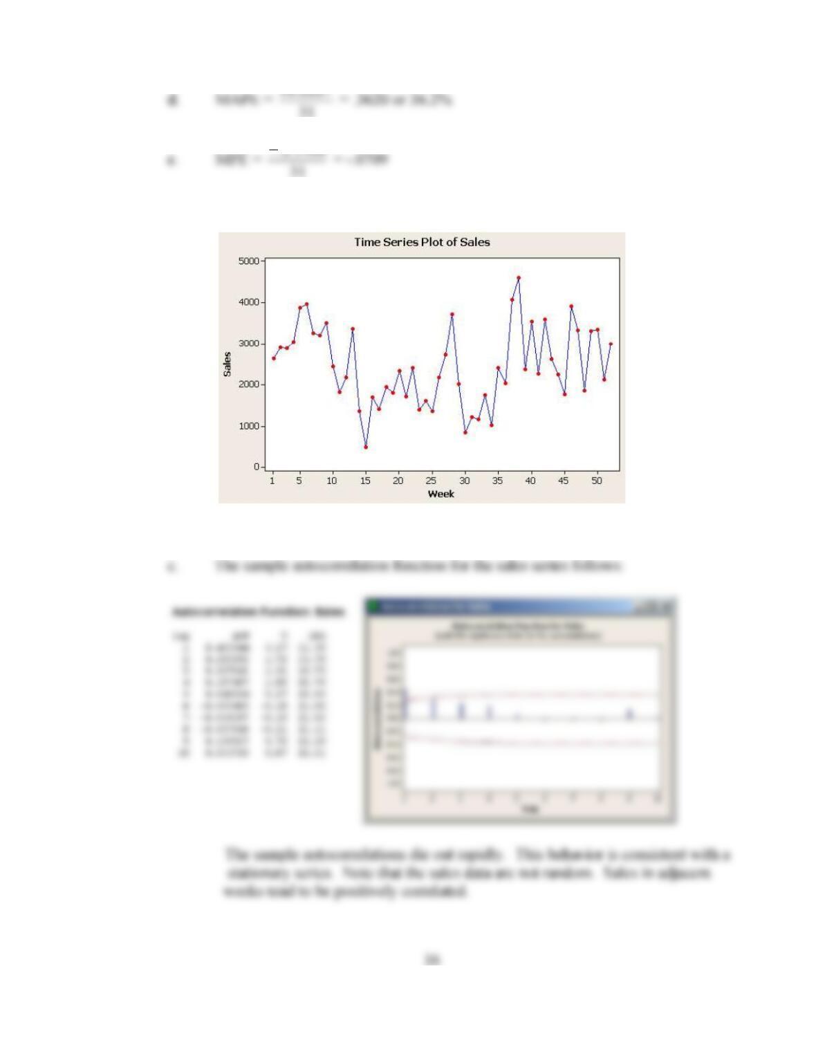
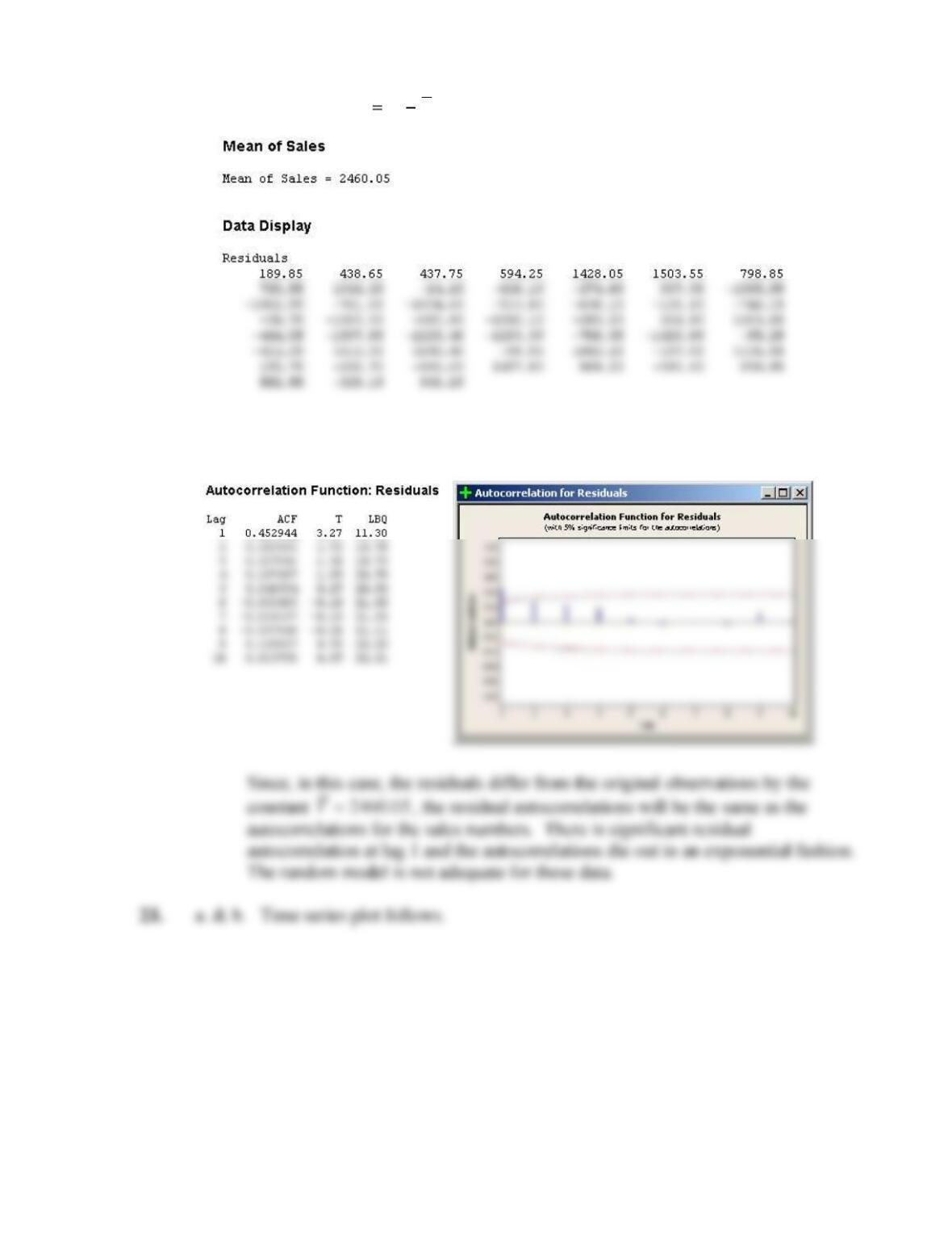
21. a. Time series plot follows
b. The sales time series appears to vary about a fixed level so it is stationary.
17
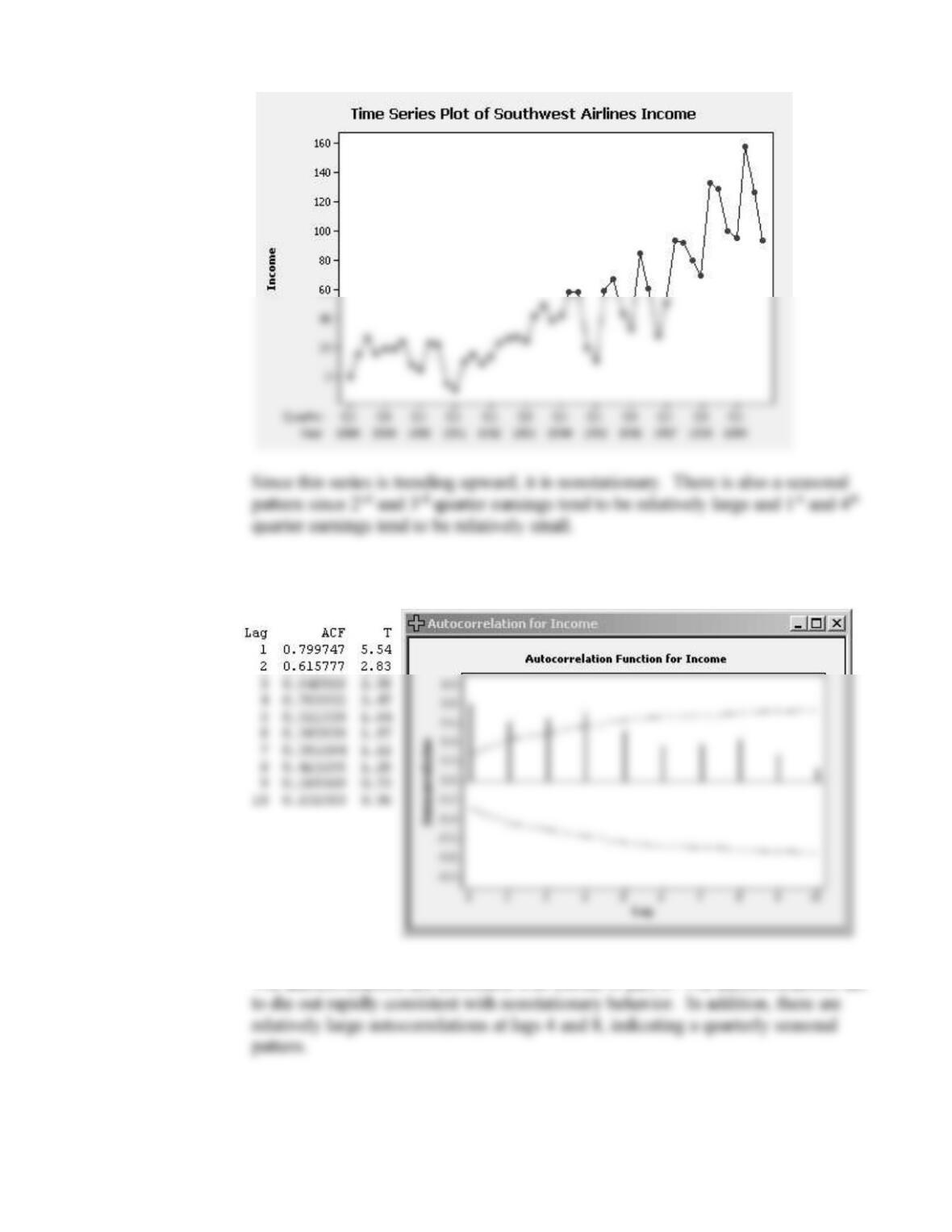
22. a. The residuals
YYe
tt are listed below
b. The residual autocorrelations follow
18
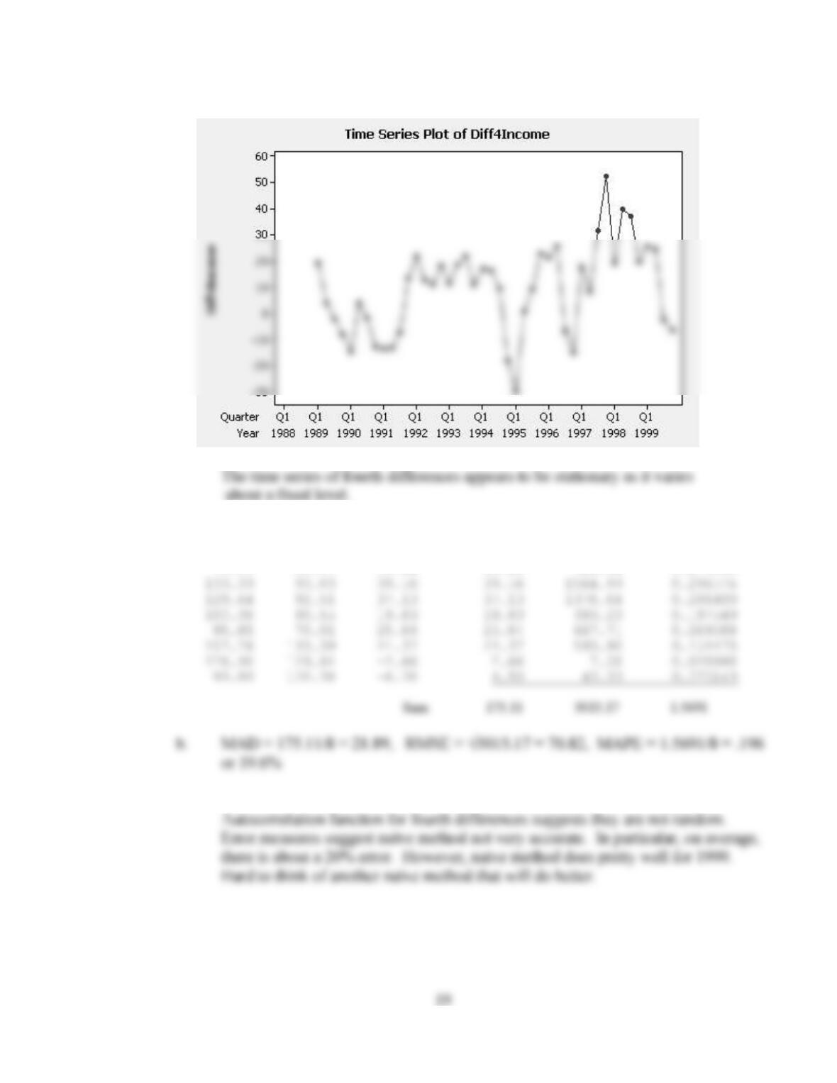
c. The autocorrelation function for the first 10 lags follows.
The autocorrelations are consistent with choice in part b. The autocorrelations fail
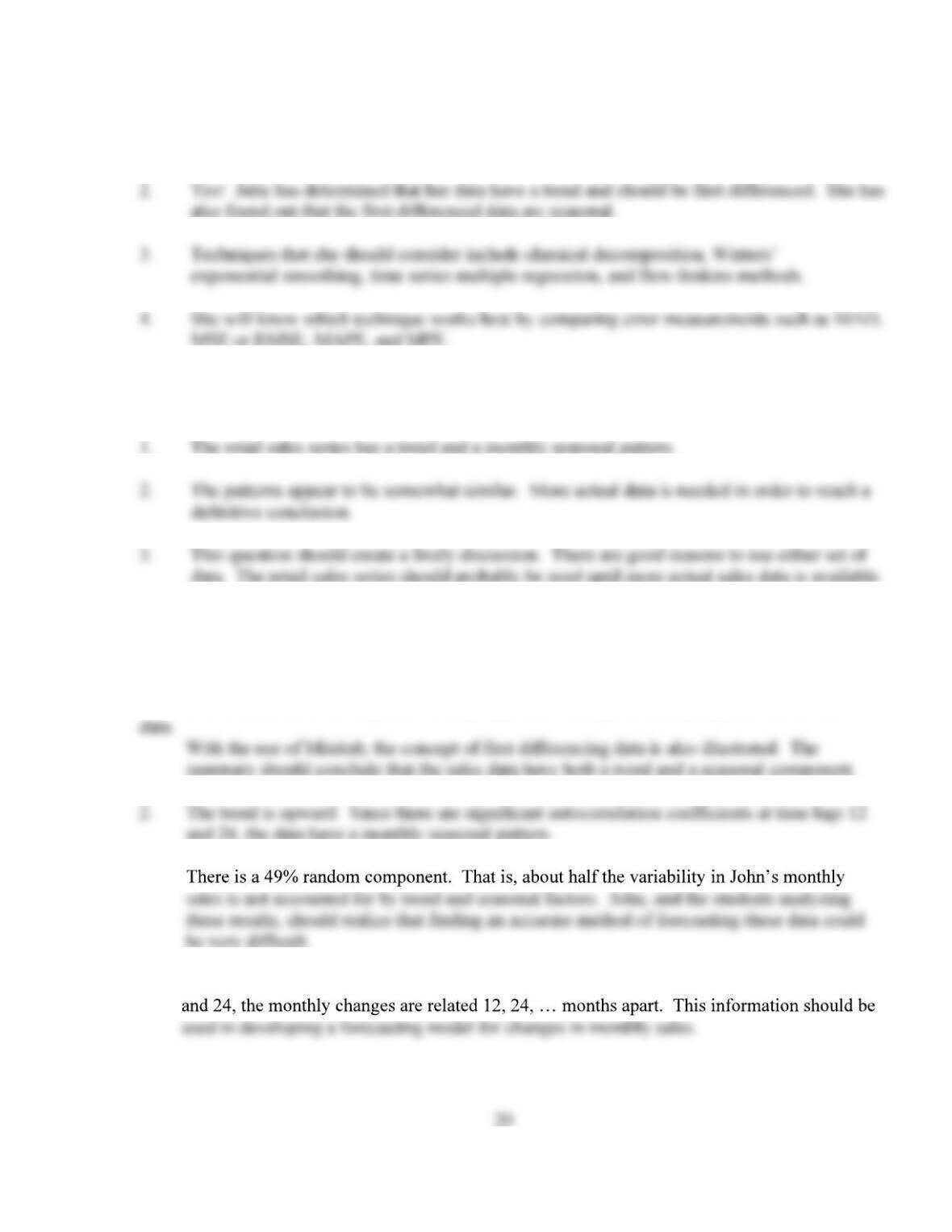
24. a. & b. Time series plot of fourth differences follows.
25. a. 98/99Inc 98/99For 98/99Err 98/99AbsErr 98/99Err^2 98/99AbE/Inc
70.01 50.87 19.14 19.14 366.34 0.273390
c. Naïve forecasting method of part a assumes fourth differences are random.
CASE 3-1A: MURPHY BROTHERS FURNITURE
1. The retail sales series has a trend and a monthly seasonal pattern.
CASE 3-1B: MURPHY BROTHERS FURNITURE
CASE 3-2: MR. TUX
1. This case affords students an opportunity to learn about the use of autocorrelation functions,
and to continue following John Mosby’s quest to find a good forecasting method for his
3.
4. Yes, the first differences have a seasonal component. Given the autocorrelations at lags 12
CASE 3-3: CONSUMER CREDIT COUNSELING
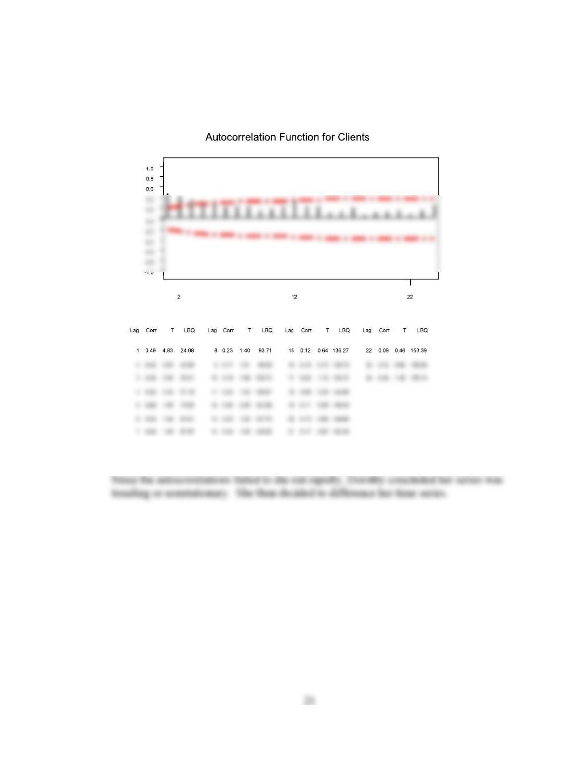
1. First, Dorothy used Minitab to compute the autocorrelation function for the number of new
clients. The results are shown below.
22
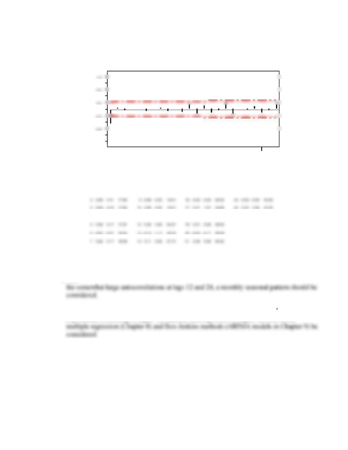
The autocorrelations for the first differenced series are:
22
12
2
0.8
0.4
0.0
-0.4
-0.8
-1.0
LBQ
T
Corr
Lag
LBQ
T
Corr
Lag
LBQ
T
Corr
Lag
LBQ
T
Corr
Lag
41.93
38.93
29.32
19.67
18.49
17.83
17.43
-0.92
-1.41
-0.93
-0.69
0.26
0.10
-4.11
-0.12
-0.18
-0.12
-0.08
0.03
0.01
-0.42
22
18
15
11
8
4
1
Autocorrelations for Differenced Data
2. The differences appear to be stationary and are correlated in consecutive time periods.
Given
3. Dorothy would recommend that various seasonal techniques such as Winters method of
exponential smoothing (Chapter 4), classical decomposition (Chapter 5), time series
23
CASE 3-4: ALOMEGA FOOD STORES
The sales data from Chapter 1 for the Alomega Food Stores case are reprinted in Case
3-4. The case suggests that Julie look at the data pattern for her sales data.
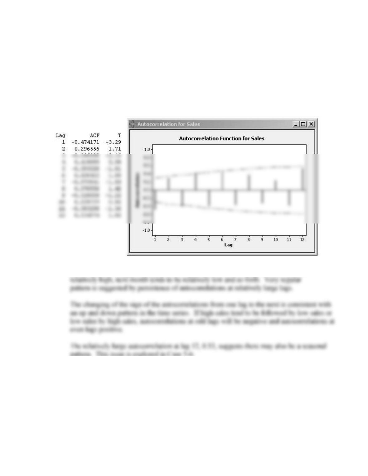
The autocorrelation function for sales follows.
Autocorrelations suggest an up and down pattern that is very regular. If one month is
CASE 3-5: SURTIDO COOKIES
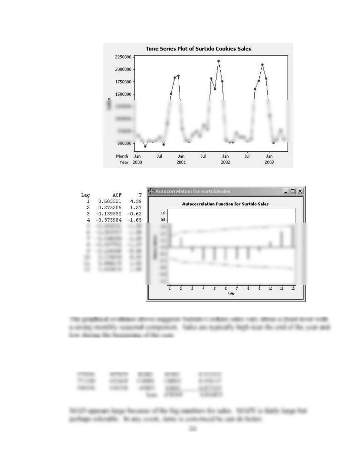
1. A time series plot and the autocorrelation function for Surtido Cookies sales follow.
2. 03Sales NaiveFor Err AbsErr AbsE/03Sales MAD = 678369/5 = 135674
1072617 681117 391500 391500 0.364995 MAPE = .816833/5 = .163 or 16.3%
510005 549689 -39684 39684 0.077811