Conjugate Gradient Method 1
3.9 Conjugate Gradient Method
In Exercises 1 – 4, solve the indicated linear system using the conjugate gradient
method in exact arithmetic. Show that the exact solution is obtained in each
case in three or fewer iterations.
1.
3x1−x2+ 2x3=−6
−x1+ 3x2+x3= 3
2x1+x2+ 3x3=−4
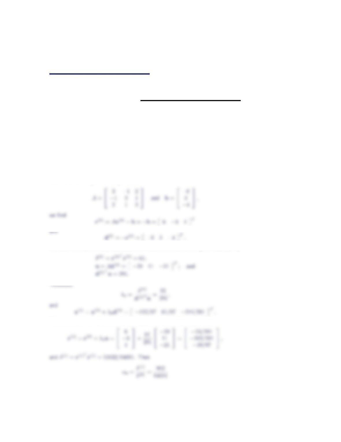
Let’s take x(0) =000T. With
We have three preliminary calculations to make before determining the step size λ0:
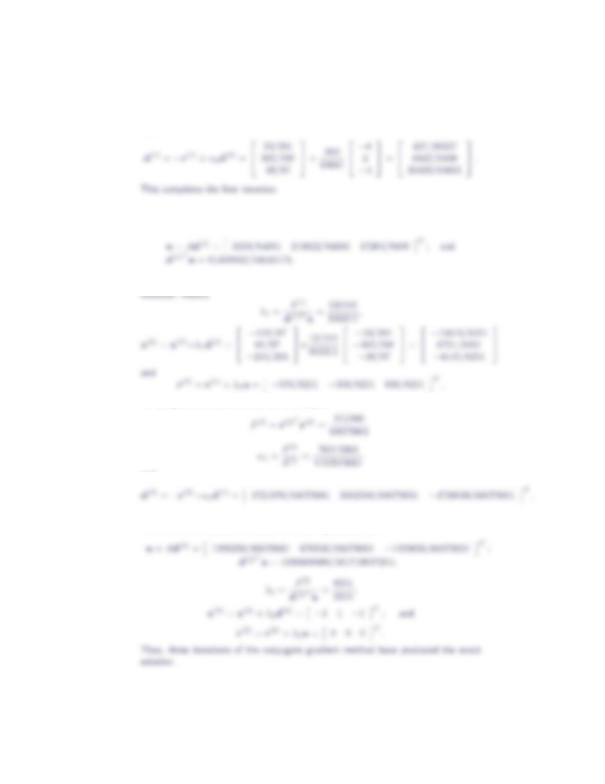
The residual associated with this new approximate solution is given by
2Section 3.9
and
To start the second iteration, only two preliminary calculations are needed to deter-
mine the step size λ1:
Recall that the value δ(1) =r(1)Tr(1) = 55022/84681 is available from the first
To complete the second iteration we compute
and
For the third iteration, we make the following calculations:
Conjugate Gradient Method 3
2.
4x1−x2= 2
−x1+ 4x2−x3= 4
−x2+ 4x3= 10
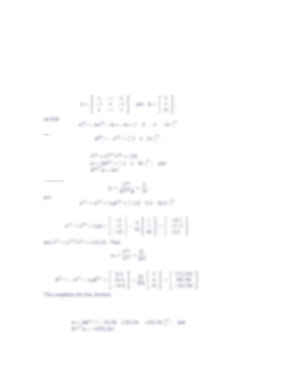
Let’s take x(0) =000T. With
We have three preliminary calculations to make before determining the step size λ0:
The residual associated with this new approximate solution is given by
and
To start the second iteration, only two preliminary calculations are needed to deter-
mine the step size λ1:
4Section 3.9
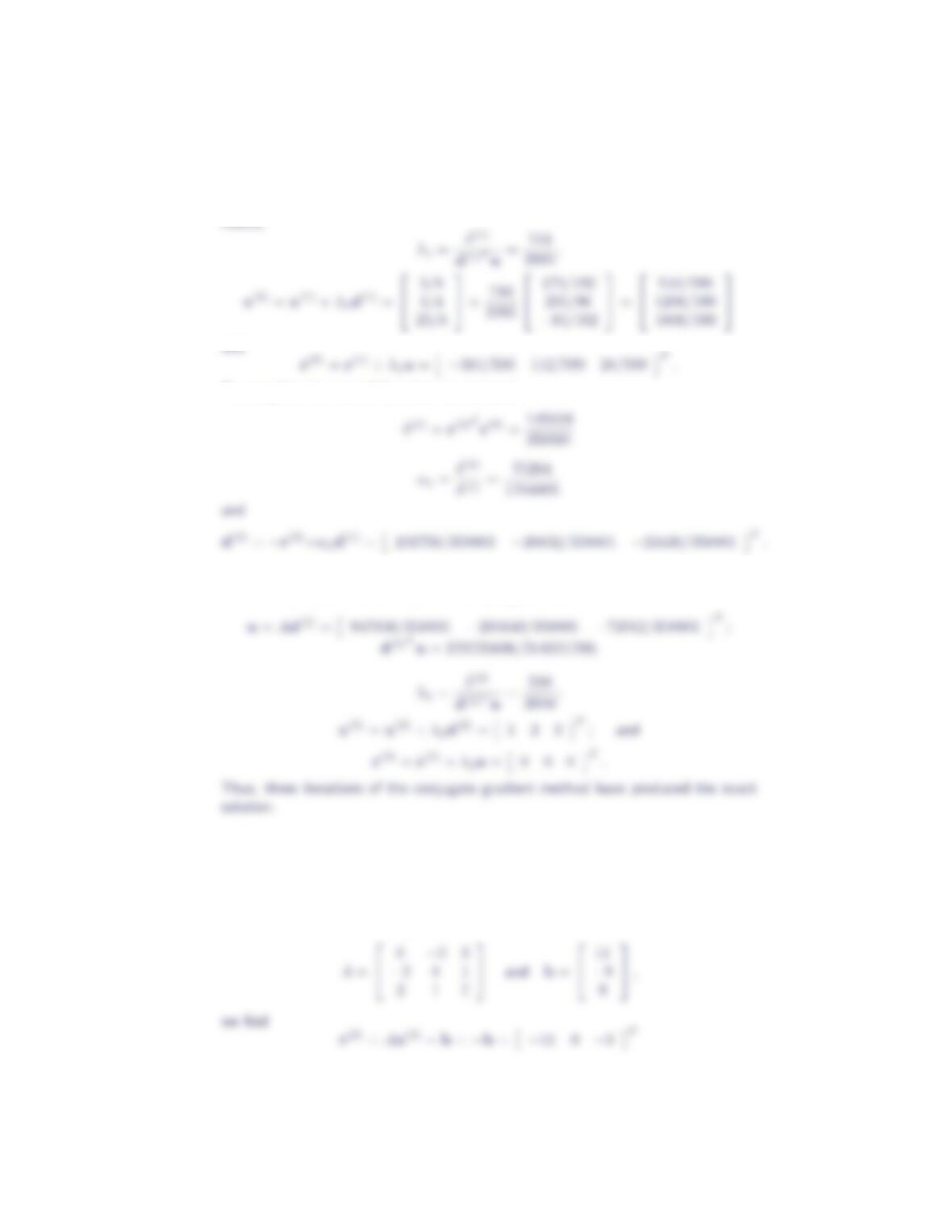
Recall that the value δ(1) =r(1)Tr(1) = 155/16 is available from the first iteration.
To complete the second iteration we compute
For the third iteration, we make the following calculations:
3.
6x1−2x2+ 3x3= 11
−2x1+ 8x2+x3=−9
3x1+x2+ 7x3= 9
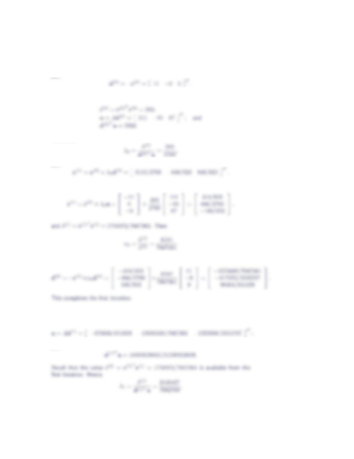
Let’s take x(0) =000T. With
Conjugate Gradient Method 5
We have three preliminary calculations to make before determining the step size λ0:
Therefore,
and
The residual associated with this new approximate solution is given by
and
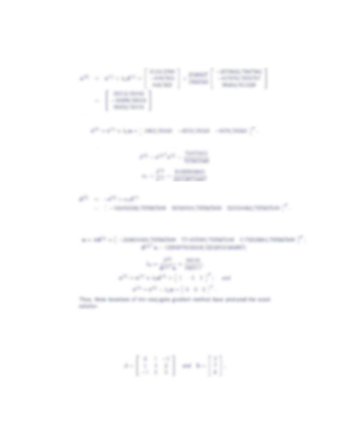
To start the second iteration, only two preliminary calculations are needed to deter-
mine the step size λ1:
and
6Section 3.9
and
To complete the second iteration we compute
and
For the third iteration, we make the following calculations:
4.
3x1+x2−x3= 2
x1+ 4x2+ 2x3= 7
−x1+ 2x2+ 5x3= 6
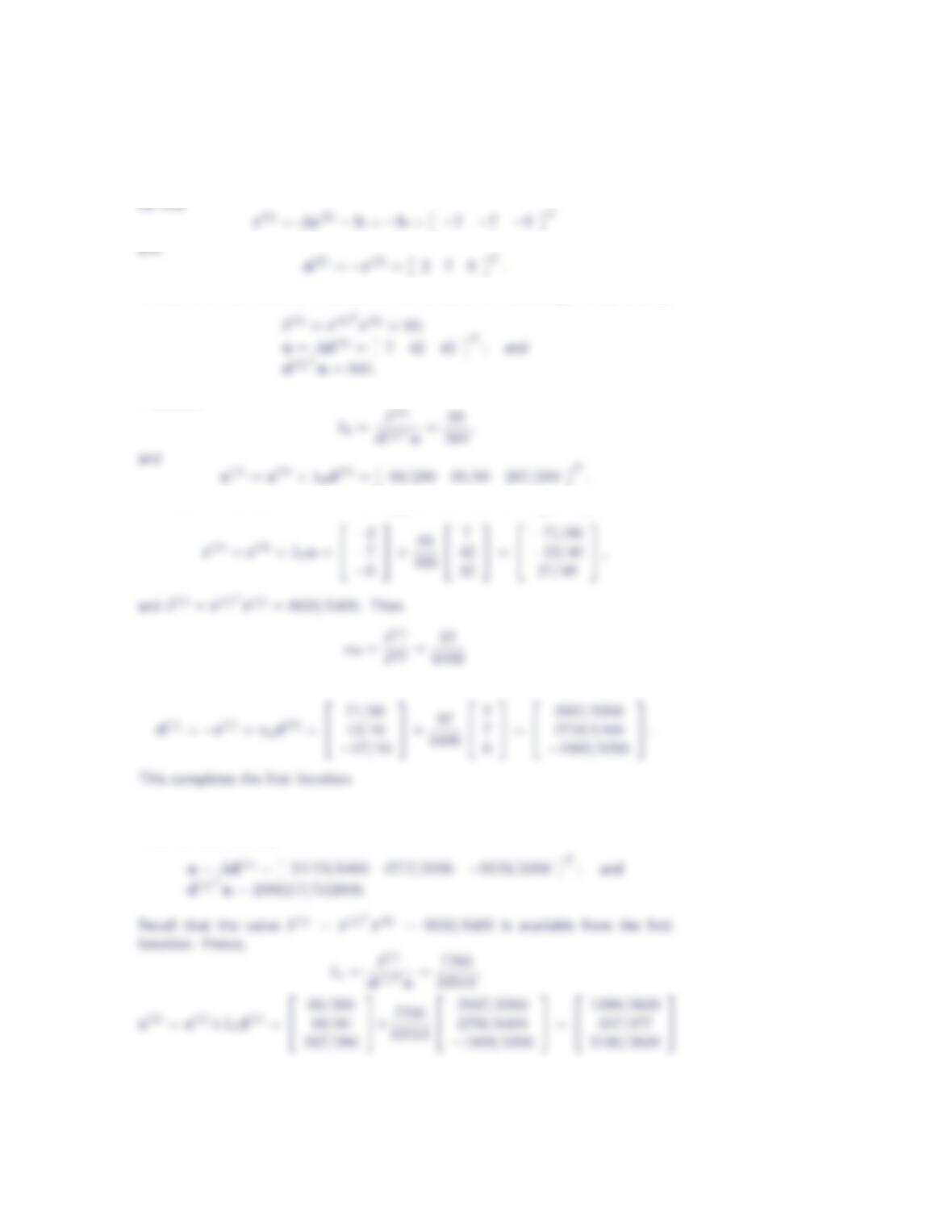
Let’s take x(0) =000T. With
Conjugate Gradient Method 7
We have three preliminary calculations to make before determining the step size λ0:
Therefore,
The residual associated with this new approximate solution is given by
and
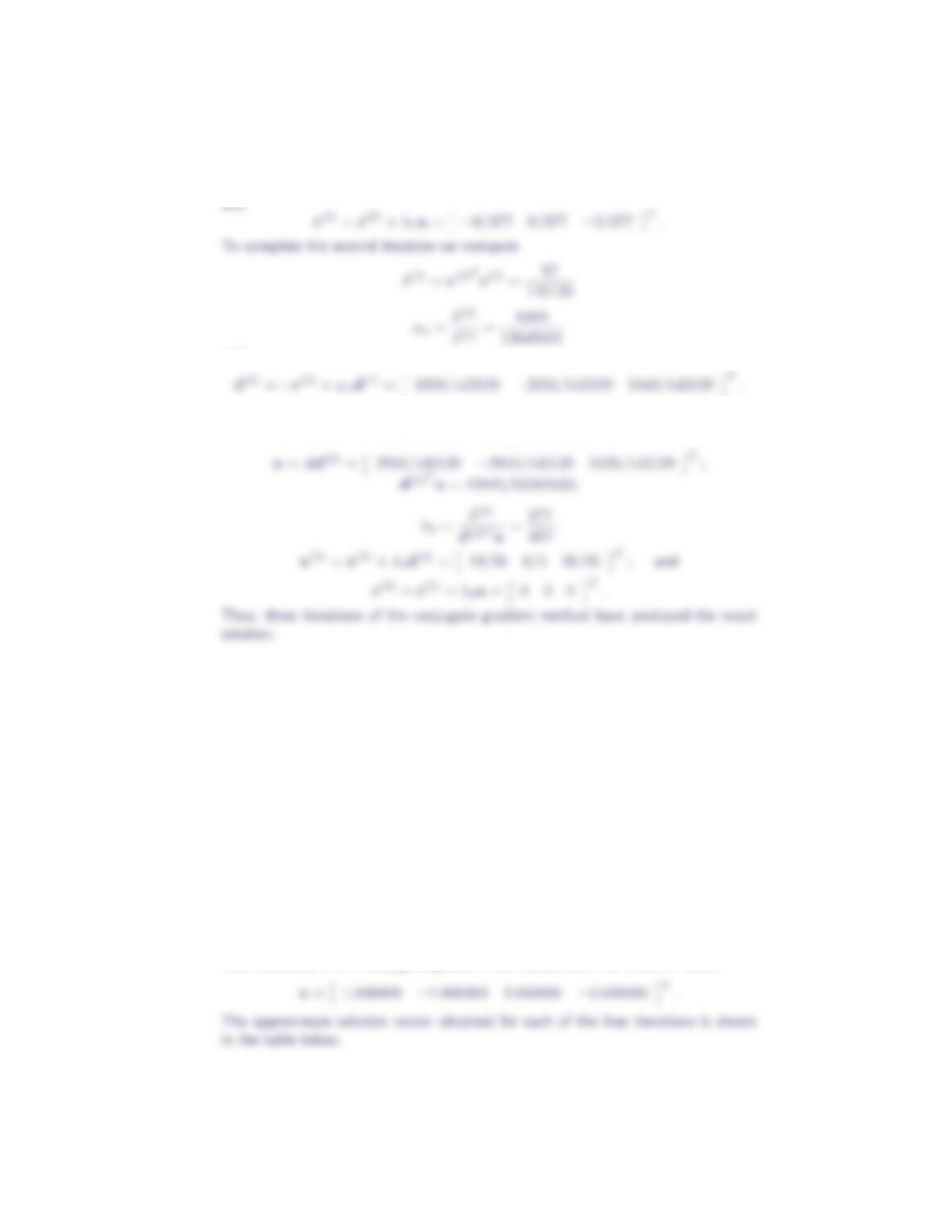
To start the second iteration, only two preliminary calculations are needed to deter-
mine the step size λ1:
8Section 3.9
and
For the third iteration, we make the following calculations:
In Exercises 5 – 10, use the conjugate gradient method to solve the indicated
linear system of equations. Take x(0) =0, and use a convergence tolerance of
5×10⁻⁷. Compare the number of iterations required to achieve convergence
with the number of iterations required by the Jacobi method and the Gauss-
Seidel method using the same starting vector and convergence tolerance. For
Exercises 7 and 8, also determine the number of iterations required by the SOR
method. The optimal values of the relaxation parameter for Exercises 7 and 8
are ω= 1.0923 and ω= 1.1128, respectively.
5.
4x1+x2+x3−x4= 8
x1+ 8x2+ 2x3+ 3x4=−12
x1+ 2x2+ 5x3−2x4= 15
−x1+ 3x2−2x3+ 4x4=−20
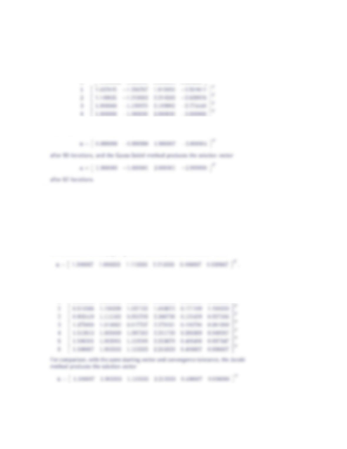
Four iterations of the conjugate gradient method produce the solution vector
Conjugate Gradient Method 9
kx(k)
00.000000 0.000000 0.000000 0.000000 T
For comparison, with the same starting vector and convergence tolerance, the Jacobi
method produces the solution vector
6.
3x1−x3−x5= 3
4x2+x3+ 2x6= 7
−x1+x2+ 5x3x6= 6
6x4−x5−2x6= 11
−x1−x4+ 7x5+ 2x6= 1
2x2+x3−2x4+ 2x5+ 8x6= 7
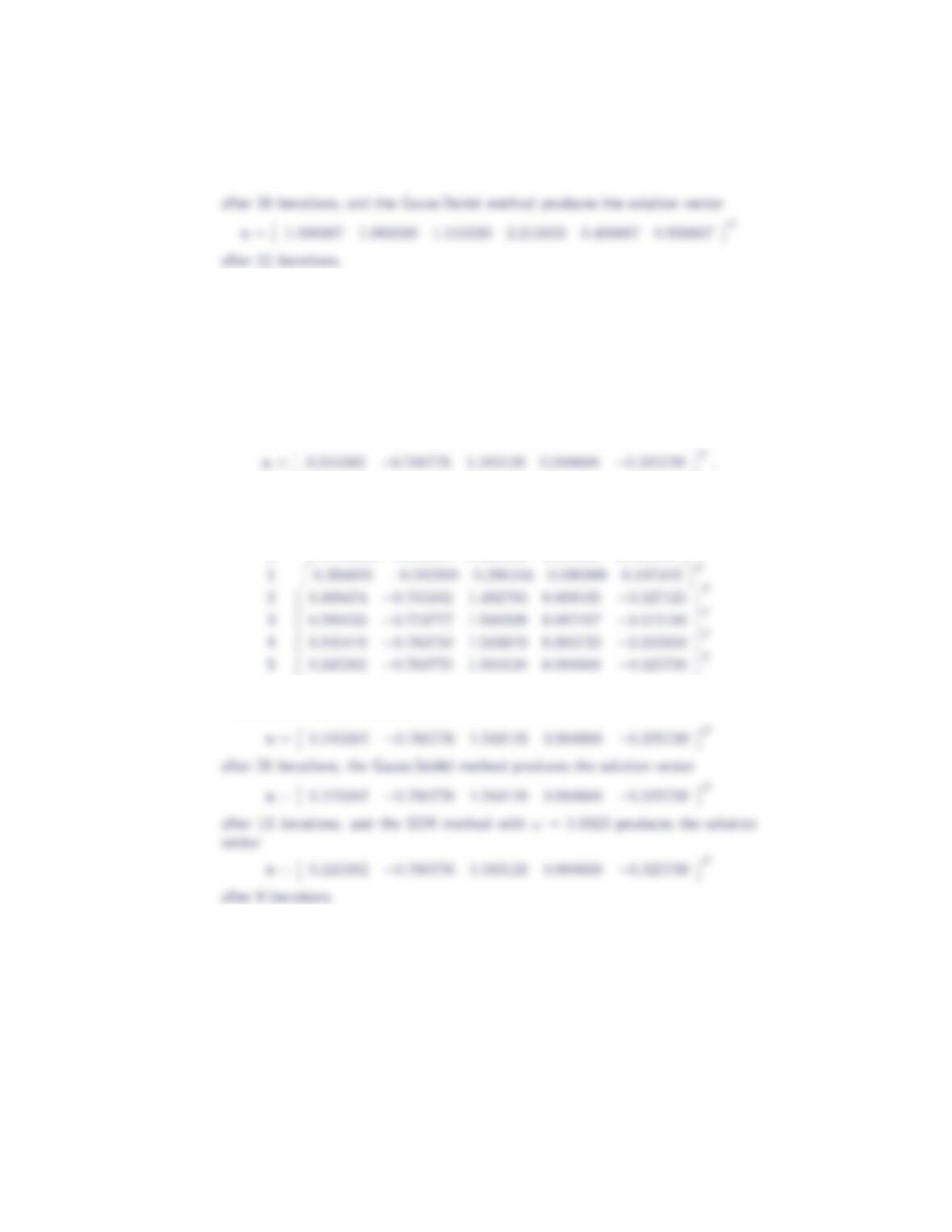
Six iterations of the conjugate gradient method produce the solution vector
The approximate solution vector obtained for each of the six iterations is shown in
the table below.
kx(k)
00.000000 0.000000 0.000000 0.000000 0.000000 0.000000 T
10 Section 3.9
7.
7x1−3x2= 4
−3x1+ 9x2+x3=−6
x2+ 3x3−x4= 3
−x3+ 10x4+ 4x5= 7
4x4+ 6x5= 2
Five iterations of the conjugate gradient method produce the solution vector
The approximate solution vector obtained for each of the five iterations is shown in
the table below.
kx(k)
00.000000 0.000000 0.000000 0.000000 0.000000 T
For comparison, with the same starting vector and convergence tolerance, the Jacobi
method produces the solution vector
8.
4x1−x2−x4=−1
−x1+ 4x2−x3−x5= 0
−x2+ 4x3−x6= 1
−x1+ 4x4−x5=−2
−x2−x4+ 4x5−x6= 1
−x3−x5+ 4x6= 2
Conjugate Gradient Method 11
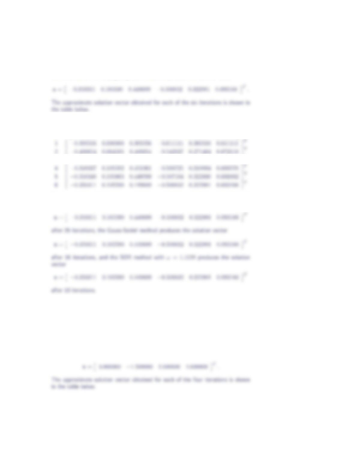
Six iterations of the conjugate gradient method produce the solution vector
kx(k)
00.000000 0.000000 0.000000 0.000000 0.000000 0.000000 T
3−0.371859 0.075377 0.452261 −0.522613 0.301508 0.673367 T
For comparison, with the same starting vector and convergence tolerance, the Jacobi
method produces the solution vector
9.
4x1+x2+x3+x4= 33/2
x1+ 3x2−x3+x4= 1/2
x1−x2+ 2x3= 17/2
x1+x2+ 3x4= 27/2
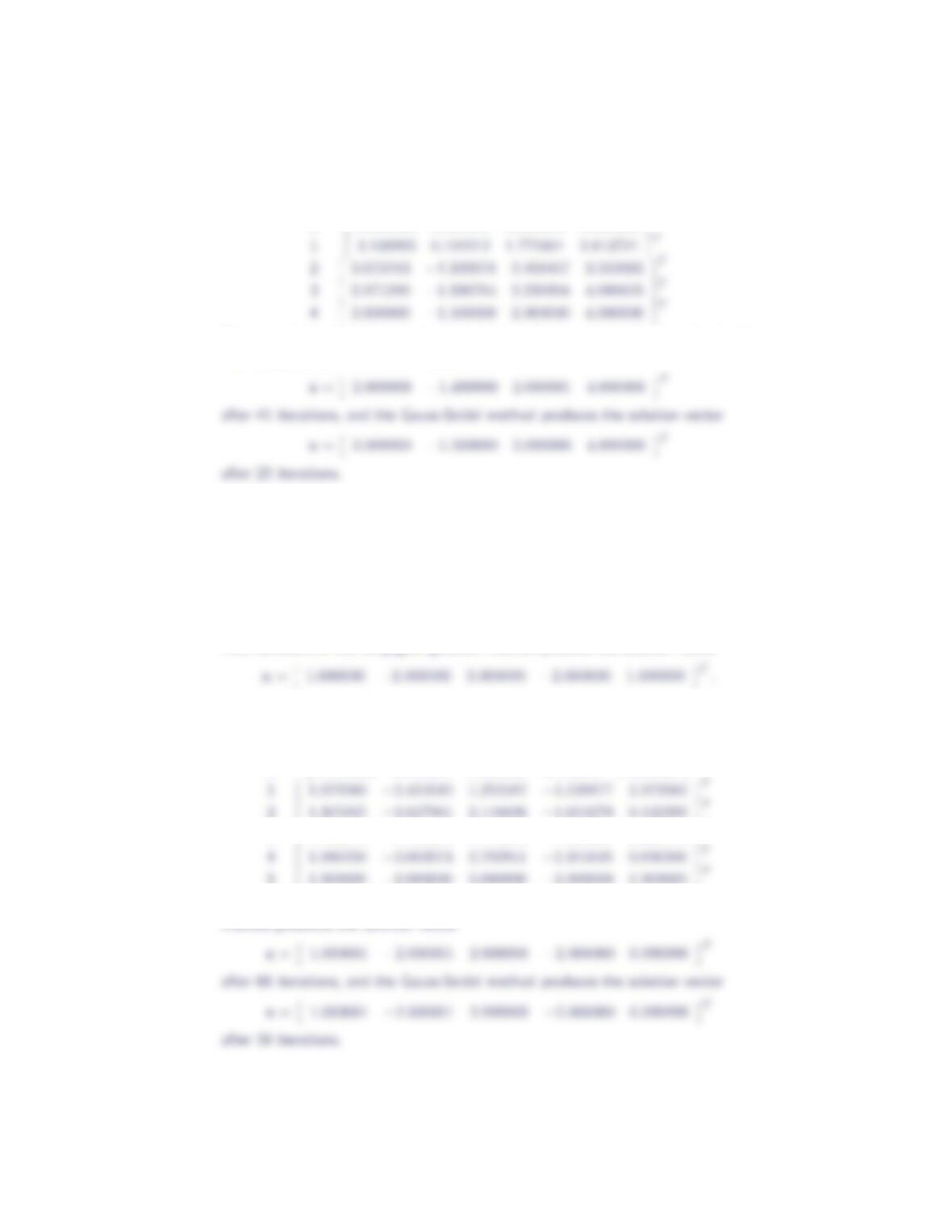
Four iterations of the conjugate gradient method produce the solution vector
12 Section 3.9
kx(k)
00.000000 0.000000 0.000000 0.000000 T
For comparison, with the same starting vector and convergence tolerance, the Jacobi
method produces the solution vector
10.
10x1+x2+ 2x3+ 3x4+ 4x5= 12
x1+ 9x2−x3+ 2x4−3x5=−27
2x1−x2+ 7x3+ 3x4−5x5= 14
3x1+ 2x2+ 3x3+ 12x4−x5=−17
4x1−3x2−5x5−x4+ 15x5= 12
Five iterations of the conjugate gradient method produce the solution vector
The approximate solution vector obtained for each of the five iterations is shown in
the table below.
kx(k)
00.000000 0.000000 0.000000 0.000000 0.000000 T
31.446618 −2.225384 2.448048 −1.970691 0.620722 T
51.000000 −2.000000 3.000000 −2.000000 1.000000 T
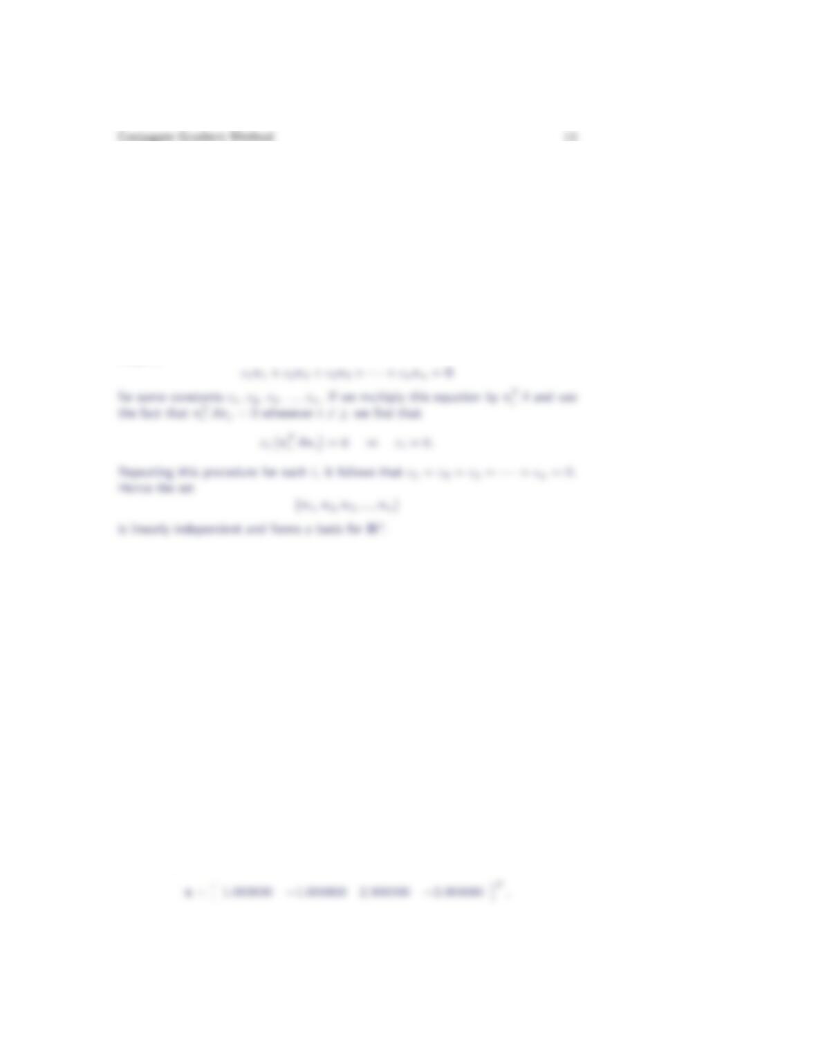
For comparison, with the same starting vector and convergence tolerance, the Jacobi
11. Let Abe an n×nsymmetric and positive definite matrix and suppose that the
non-zero vectors v1,v2,v3, …, vnform an A-conjugate set; that is, vT
iAvj= 0
whenever i6=j. Show that
c1v1+c2v2+c3v3+··· +cnvn=0
requires that c1=c2=c3=··· =cn= 0. Hence the set
{v1,v2,v3, …, vn}
is linearly independent and forms a basis for Rn.
Suppose
12. A simpler choice for the search direction would be to set d(m)=−r(m). This
amounts to always selecting the direction in which fdecreases most rapidly
in the vicinity of x(m)and produces what is known as the method of steepest
descent. The resulting algorithm is summarized in the following pseudocode.
r(0) =Ax(0) −b
for m= 0, 1, 2, …
d(m)=−r(m)
λm=−d(m)Tr(m)/d(m)TAd(m)
x(m+1) =x(m)+λmd(m)
r(m+1) =r(m)+λmAd(m)
if √r(m+1)Tr(m+1) < T OL, OUTPUT x(m+1)
Solve the linear systems in Exercises 5 – 10 using the method of steepest descent
with x(0) =0and a convergence tolerance of 5×10⁻⁷. Compare the performance
of the method of steepest descent with that of the conjugate gradient method.
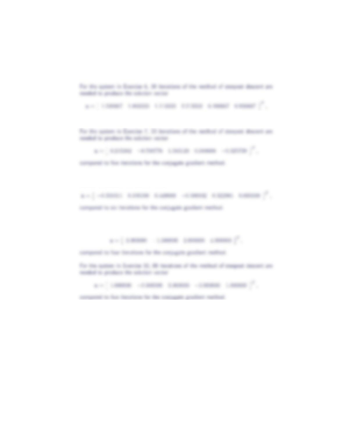
For the system in Exercise 5, 121 iterations of the method of steepest descent are
needed to produce the solution vector
14 Section 3.9
compared to four iterations for the conjugate gradient method.
compared to six iterations for the conjugate gradient method.
For the system in Exercise 8, 28 iterations of the method of steepest descent are
needed to produce the solution vector
For the system in Exercise 9, 50 iterations of the method of steepest descent are
needed to produce the solution vector
13. The coefficients of the least squares cubic polynomial a0+a1x+x2x2+a3x3
which fits the data
x0 0.5 1.0 1.5 2.0 2.5 3.0 3.5
y1.0 1.7 2.1 2.0 1.1 0.9 1.4 3.1
satisfy the linear system of equations
8 14 35 98
14 35 98 292.25
35 98 292.25 906.5
98 292.25 906.5 2887.8125
a0
a1
a2
a3
=
13.3
25.45
67.625
202.6375
.
Conjugate Gradient Method 15
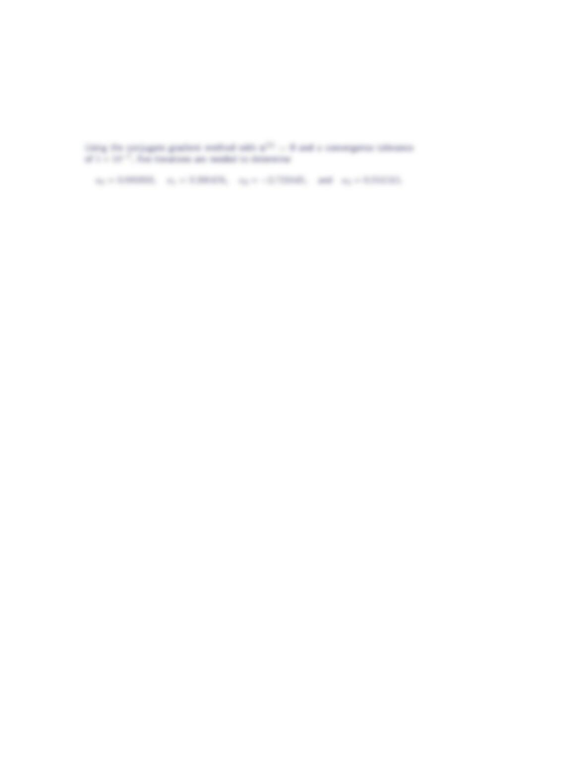
Determine the values of a0, a1, a2and a3.