Iterative Methods, Basic Concepts 13
kx(k)
00.000000 0.000000 0.000000 0.000000 0.000000 T
10.571429 −0.666667 1.000000 0.700000 0.333333 T
20.285714 −0.587302 1.455556 0.933333 0.800000 T
13 0.238154 −0.777855 1.715579 1.369809 1.246065 T
14 0.238062 −0.777902 1.715888 1.369984 1.246539 T
15 0.238042 −0.777967 1.715962 1.370204 1.246656 T
16 0.238014 −0.777982 1.716057 1.370259 1.246803 T
Twelve iterations of the Gauss-Seidel method are needed to produce the solution
vector
14 Section 3.8
kx(k)
00.000000 0.000000 0.000000 0.000000 0.000000 T
10.571429 −0.476190 1.158730 0.815873 0.877249 T
10.
4x1−x2−2x4=−1
−x1+ 4x2−x3−2x5= 0
−x2+ 4x3−2x6= 1
−x1+ 4x4−x5=−2
−x2−x4+ 4x5−x6= 1
−x3−x5+ 4x6= 2
Iterative Methods, Basic Concepts 15
kx(k)
00.000000 0.000000 0.000000 0.000000 0.000000 0.000000 T
5−0.472656 0.187500 0.660156 −0.546875 0.343750 0.734375 T
6−0.476562 0.218750 0.664062 −0.532227 0.343750 0.750977 T
17 −0.446917 0.249023 0.695940 −0.518345 0.374512 0.767369 T
18 −0.446917 0.249512 0.695940 −0.518101 0.374512 0.767613 T
19 −0.446673 0.249512 0.696184 −0.518101 0.374756 0.767613 T
20 −0.446673 0.249756 0.696184 −0.517979 0.374756 0.767735 T
21 −0.446551 0.249756 0.696307 −0.517979 0.374878 0.767735 T
Eighteen iterations of the Gauss-Seidel method are needed to produce the solution
vector
16 Section 3.8
shown in the table below.
kx(k)
00.000000 0.000000 0.000000 0.000000 0.000000 0.000000 T
1−0.250000 −0.062500 0.234375 −0.562500 0.093750 0.582031 T
9−0.448626 0.247803 0.695330 −0.518956 0.373901 0.767308 T
10 −0.447527 0.248901 0.695879 −0.518406 0.374451 0.767582 T
11 −0.446978 0.249451 0.696154 −0.518132 0.374725 0.767720 T
12 −0.446703 0.249725 0.696291 −0.517994 0.374863 0.767788 T
11. The linear systems in Exercises 8 and 9 have positive definite, tridiagonal co-
efficient matrices. Determine the optimal value of the relaxation parameter for
the SOR method for each system. Using the corresponding optimal value of
ω, solve the systems from Exercises 8 and 9. Take x(0) =0, and terminate
iteration when kx(k+1) −x(k)k∞falls below 5 ×10⁻⁶.
For the system of equations in Exercise 8,
0 1/4 0
Iterative Methods, Basic Concepts 17
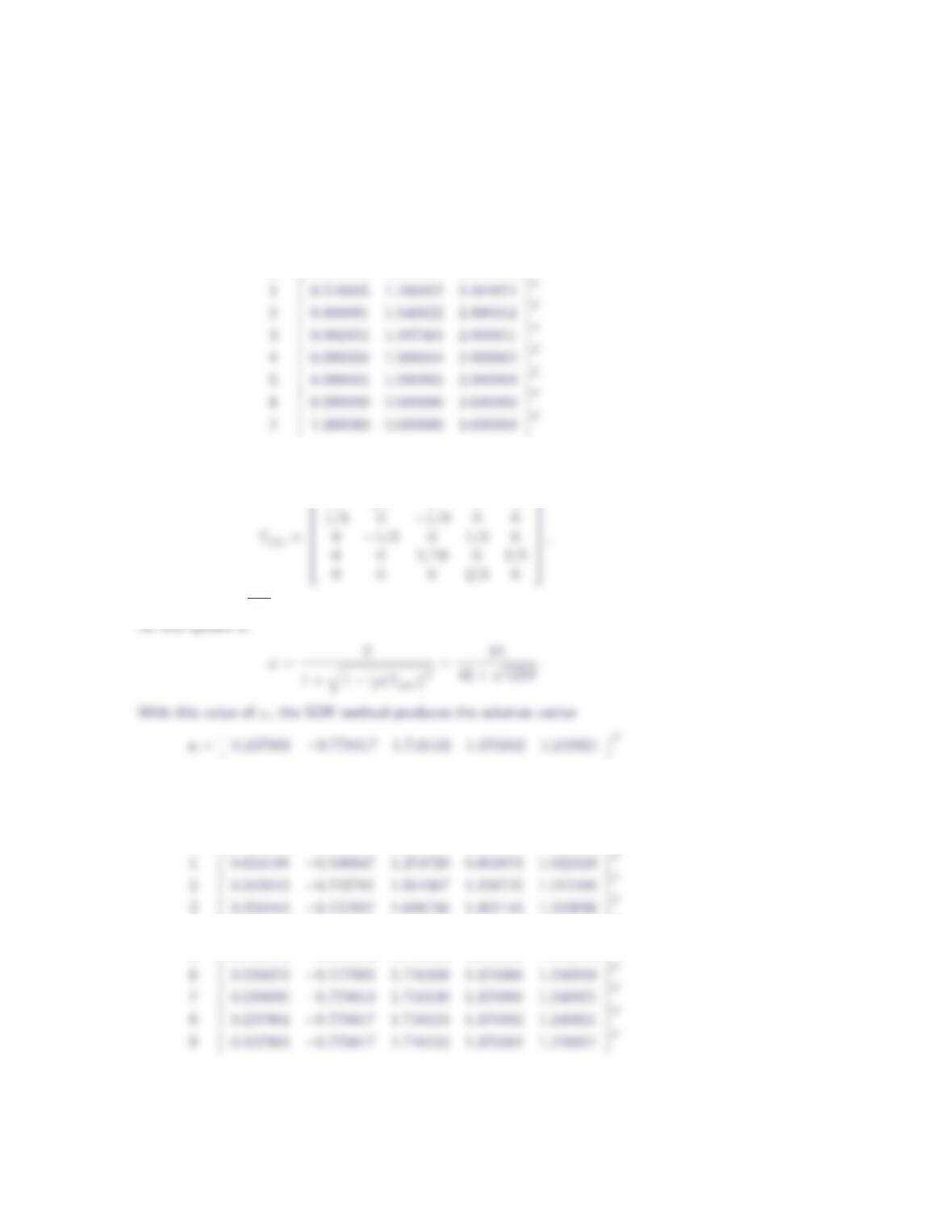
in seven iterations. The approximate solution vector obtained for each of the seven
iterations is shown in the table below.
kx(k)
00.000000 0.000000 0.000000 T
For the system of equations in Exercise 9,
0 3/7 0 0 0
and ρ(Tjac) = √546/42. Thus, the optimal value of the SOR relaxation parameter
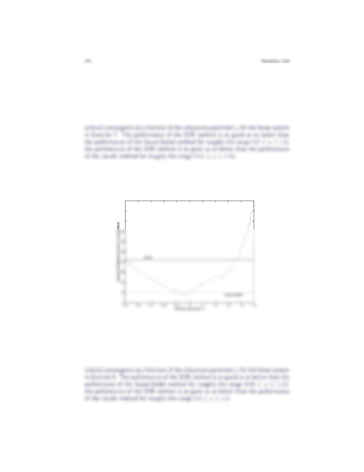
in nine iterations. The approximate solution vector obtained for each of the nine
iterations is shown in the table below.
kx(k)
00.000000 0.000000 0.000000 0.000000 0.000000 T
40.245523 −0.774779 1.713381 1.369263 1.246459 T
50.238813 −0.777683 1.715858 1.370253 1.246870 T
12. For each of the linear systems in Exercises 7 – 10, generate a plot of the number
of iterations required by the SOR method to achieve convergence as a function
of the relaxation parameter ω. Take x(0) =0, and terminate iteration when
kx(k+1) −x(k)k∞falls below 5×10⁻⁶. Over roughly what range of ωvalues does
the SOR method outperform the Gauss-Seidel method? the Jacobi method?
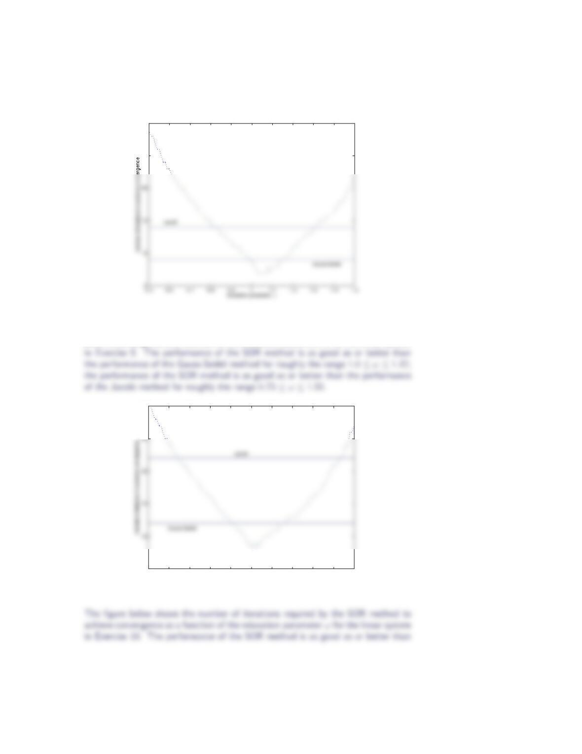
The figure below shows the number of iterations required by the SOR method to
45
50
55
The figure below shows the number of iterations required by the SOR method to
Iterative Methods, Basic Concepts 19
25
30
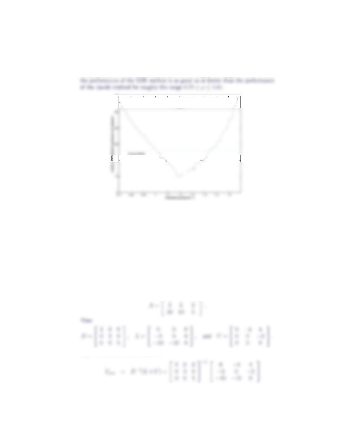
The figure below shows the number of iterations required by the SOR method to
achieve convergence as a function of the relaxation parameter ωfor the linear system
0.6 0.7 0.8 0.9 11.1 1.2 1.3 1.4 1.5 1.6
5
30
relaxation parameter, !
20 Section 3.8
the performance of the Gauss-Seidel method for roughly the range 1.0≤ω≤1.45;
15
35
Jacobi
13. Let
A=
2 4 −4
3 3 3
10 10 5
.
(a) Write out the iteration matrix Tjac corresponding to the matrix A, and
determine ρ(Tjac). Will the Jacobi method converge for any choice of the
initial vector x(0)?
(b) Write out the iteration matrix Tgs corresponding to the matrix A, and
determine ρ(Tgs). Will the Gauss-Seidel method converge for any choice
of the initial vector x(0)?
Let
2 4 −4
(a) The Jacobi iteration matrix is
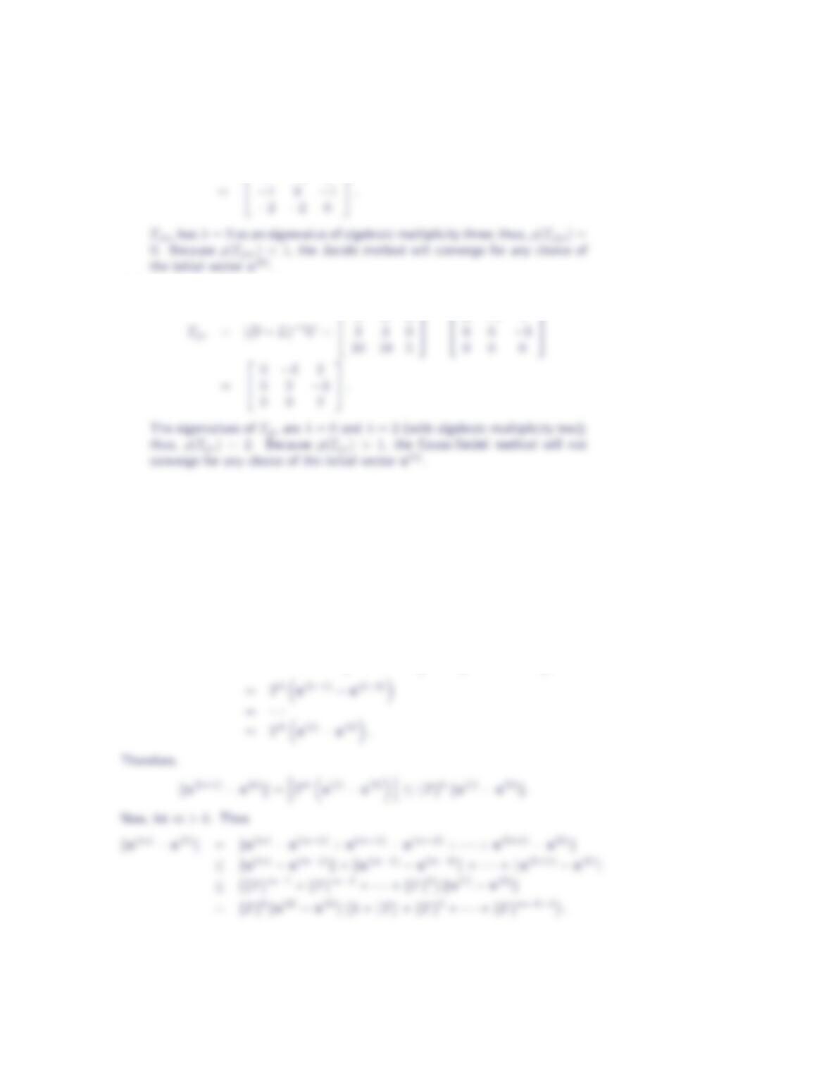
Iterative Methods, Basic Concepts 21
0−2 2
(b) The Gauss-Seidel iteration matrix is
2 0 0
−1
0−4 4
14. Consider the iteration scheme x(k+1) =Tx(k)+c, and suppose that kTk<1
for some natural matrix norm. Show that for any x(0) ∈Rn:
kx−x(k)k ≤ kTkk
1− kTkkx(1) −x(0)k.
(Hint: Review the proof of the fixed point iteration convergence theorem in
Section 2-3).
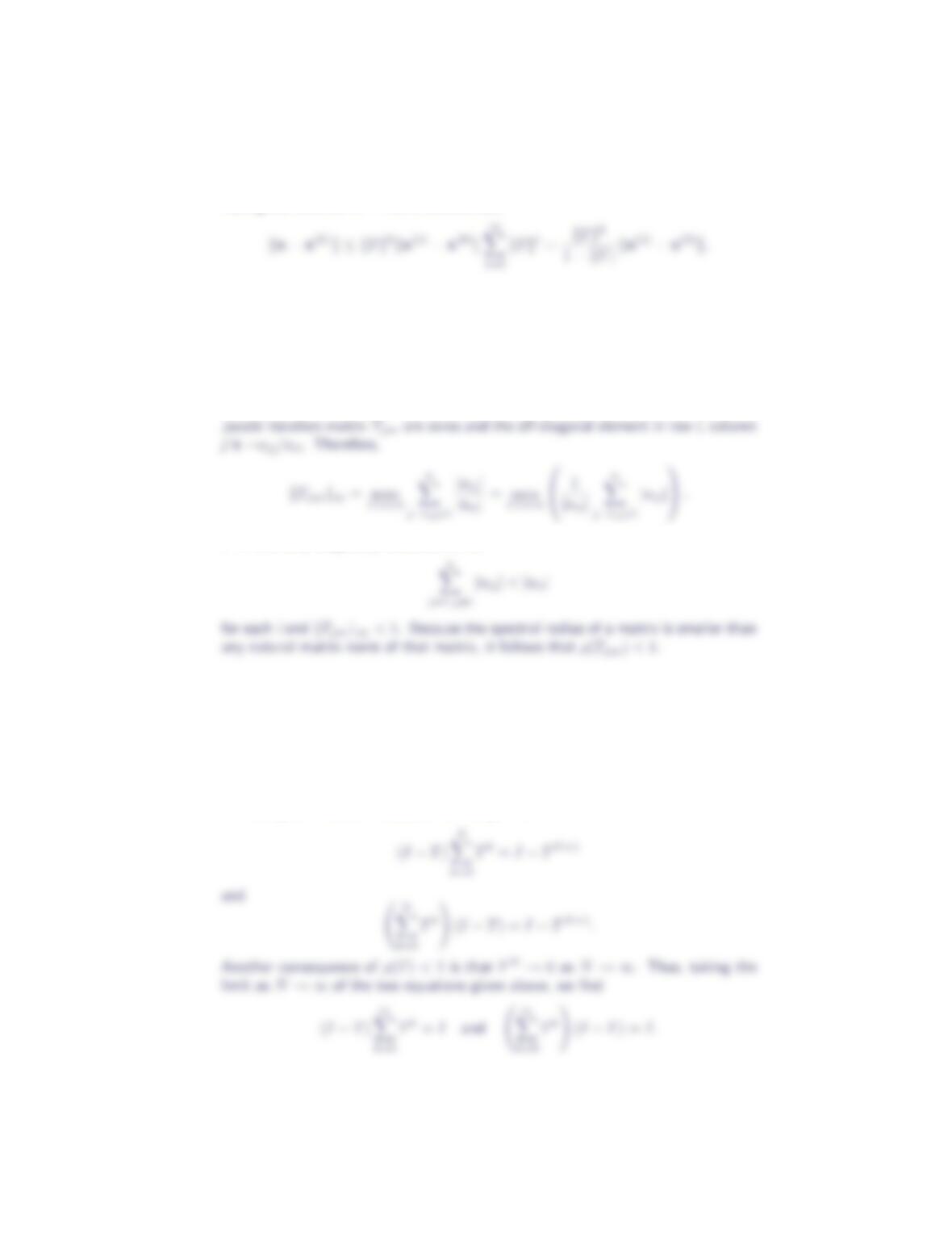
We start by noting that
x(k+1) −x(k)=Tx(k)+c−Tx(k−1) +c=Tx(k)−x(k−1)
22 Section 3.8
Taking the limit as m→ ∞, it follows that
15. Let Abe a strictly diagonally dominant matrix and let Tjac be the Jacobi method
iteration matrix associated with A. Show that ρ(Tjac)<1. (Hint: Show that
kTjack∞<1 and use the fact that the spectral radius of a matrix is smaller
than any natural matrix norm of that matrix.)
For an arbitrary matrix A, the elements along the diagonal of the corresponding
If Ais strictly diagonally dominant, then
16. Suppose that ρ(T)<1. Show that
(I−T)−1=
∞
X
k=0
Tk.
Because ρ(T)<1, we know from Exercise 10 in Section 3.3 that the matrix I−T
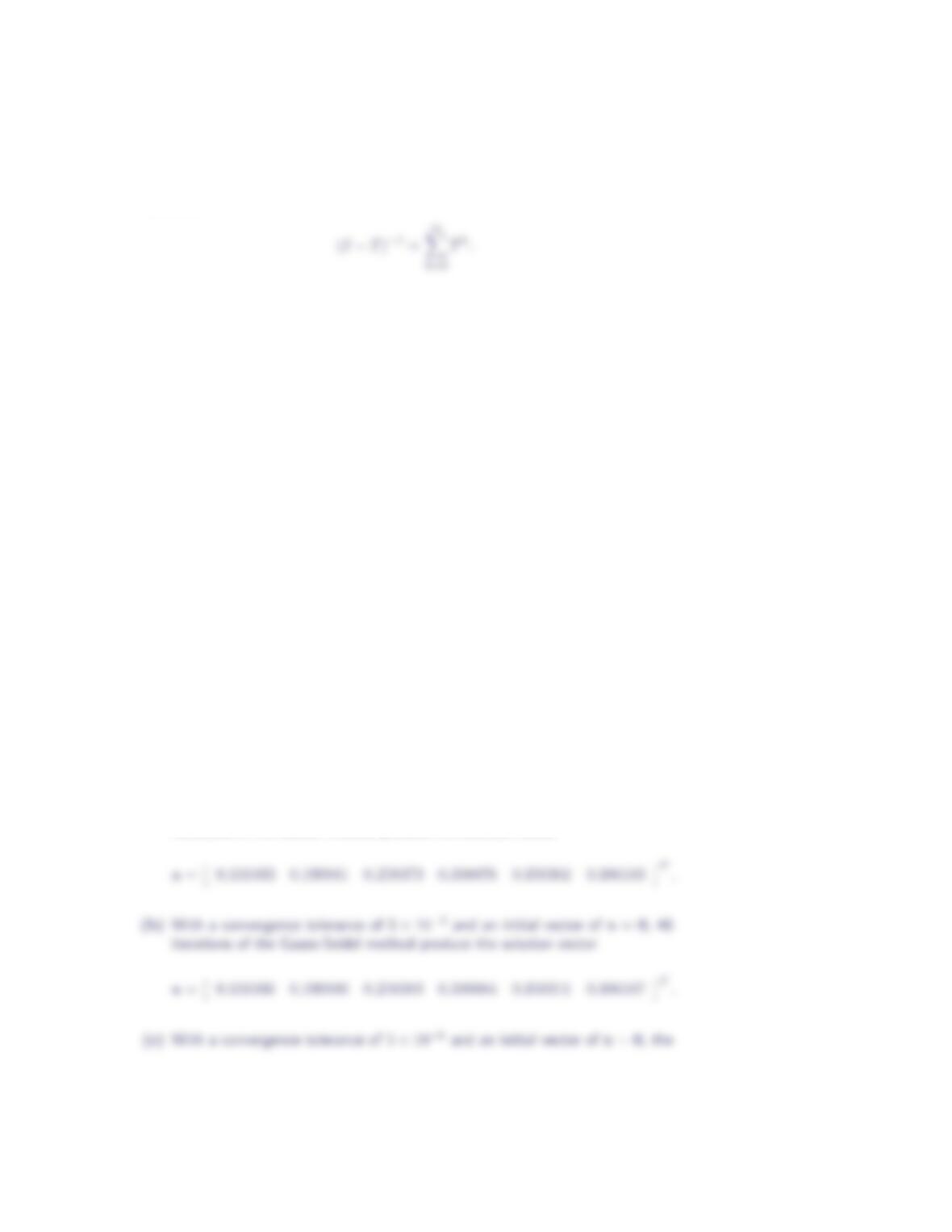
is nonsingular. Now, for any positive integer N,
Iterative Methods, Basic Concepts 23
Therefore,
17. The variables of interest in an absorption column are the steady-state composi-
tion of solute in the liquid, xi, on each plate and the steady-state composition
of the solute in the gas, yi, on each plate. Suppose we have a six plate ab-
sorption column, where the inlet compositions, x0= 0.05 kg solute/kg liquid
and y7= 0.3 kg solute/kg inert gas, are known, as are the liquid and gas flow
rates, L= 40.8 kg/min and G= 66.7 kg/min. Further, we will assume that the
linear equilibrium relationship yi= 0.72xiholds. Performing a material balance
around an arbitrary plate, we find that the xisatisfy the system
−88.824 48.024 0 0 0 0
40.8−88.824 48.024 0 0 0
0 40.8−88.824 48.024 0 0
0 0 40.8−88.824 48.024 0
0 0 0 40.8−88.824 48.024
0 0 0 0 40.8−88.824
x1
x2
x3
x4
x5
x6
=
−2.04
0
0
0
0
−20.01
.
Determine the xiusing
(a) the Jacobi method;
(b) the Gauss-Seidel method; and
(c) the SOR method with ωranging from 1.1 through 1.9 in increments of 0.1.
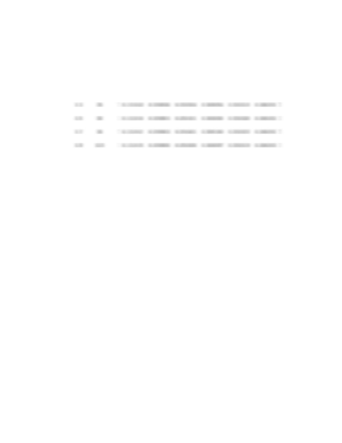
(a) With a convergence tolerance of 5×10⁻⁶and an initial vector of x=0, 89
iterations of the Jacobi method produce the solution vector
24 Section 3.8
following results were obtained from the SOR method:
ωiterations xT
1.1 39 0.131037 0.199887 0.258385 0.308086 0.350313 0.386188
1.2 32 0.131040 0.199892 0.258391 0.308091 0.350316 0.386190
1.4 15 0.131047 0.199902 0.258400 0.308099 0.350321 0.386192
1.6 27 0.131047 0.199902 0.258399 0.308098 0.350320 0.386192
1.8 56 0.131047 0.199902 0.258400 0.308098 0.350320 0.386190