14
Problem 3.14
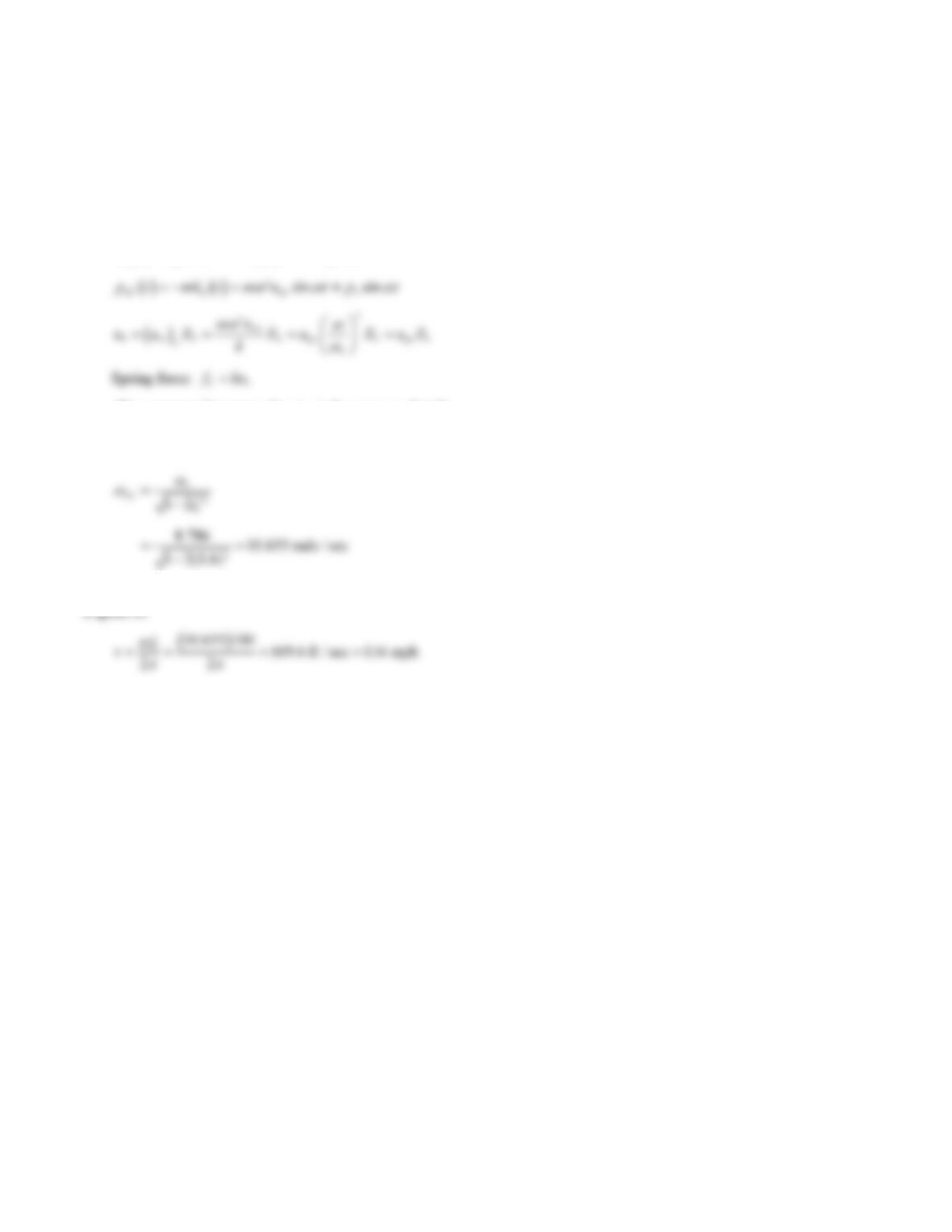
Determine the speed of the automobile in Example 3.4 that
would produce a resonant condition for the spring force in
the suspension system.
Solution:
2
sin sin
ggoggo
ut u t ut u t
The resonant frequency for fS is the same as that for
uo, which is the resonant frequency for Ra (from Section
3.2.5):
Resonance occurs at this forcing frequency, which implies
a speed of
15
Problem 3.15
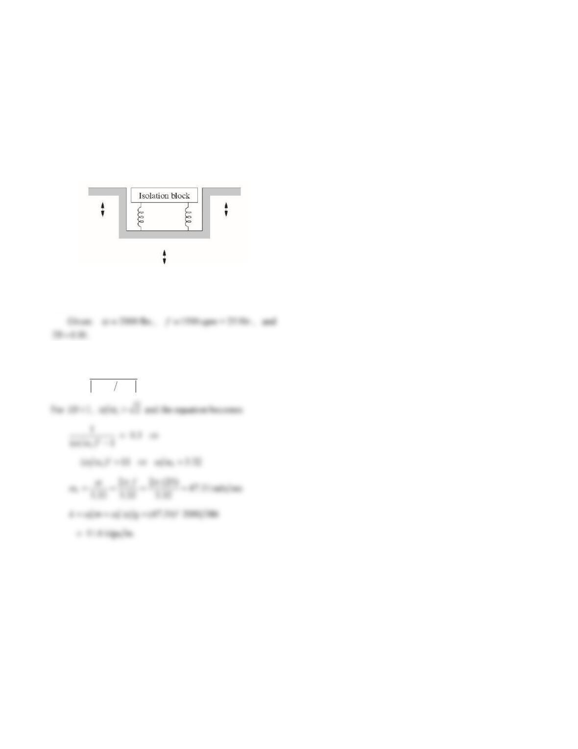
A vibration isolation block is to be installed in a laboratory
so that the vibration from adjacent factory operations will
not disturb certain experiments (Fig. P3.15). If the isolation
block weighs 2000 lb and the surrounding floor and foun-
dation vibrate at 1500 cycles per minute, determine the
stiffness of the isolation system such that the motion of the
isolation block is limited to 10% of the floor vibration;
neglect damping.
Figure P3.15
Solution:
For an undamped system,
2
10.1
1( )
n
TR
16
Problem 3.16
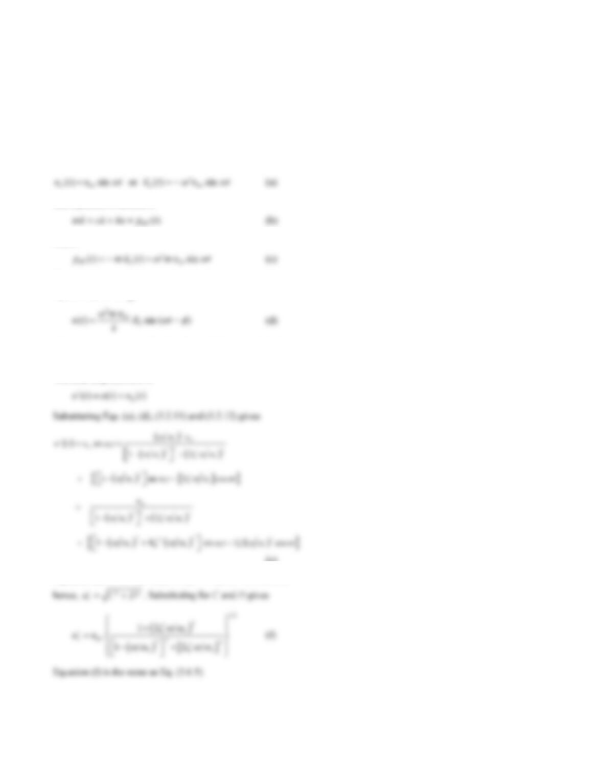
An SDF system is subjected to support displacement
ug(t) = ugo sin ωt. Show that the amplitude t
o
u of the total
displacement of the mass is given by Eq. (3.6.5).
Solution:
The excitation is
The equation of motion is
where
The deformation response is given by Eq. (3.2.10) with
p
o
replaced by
2mu
go :
where Rd and
are defined by Eqs. (3.2.11) and (3.2.12),
respectively.
The total displacement is
(e)
Equation (e) is of the form () sin cos
t
ut C t D t
;
17
Problem 3.17
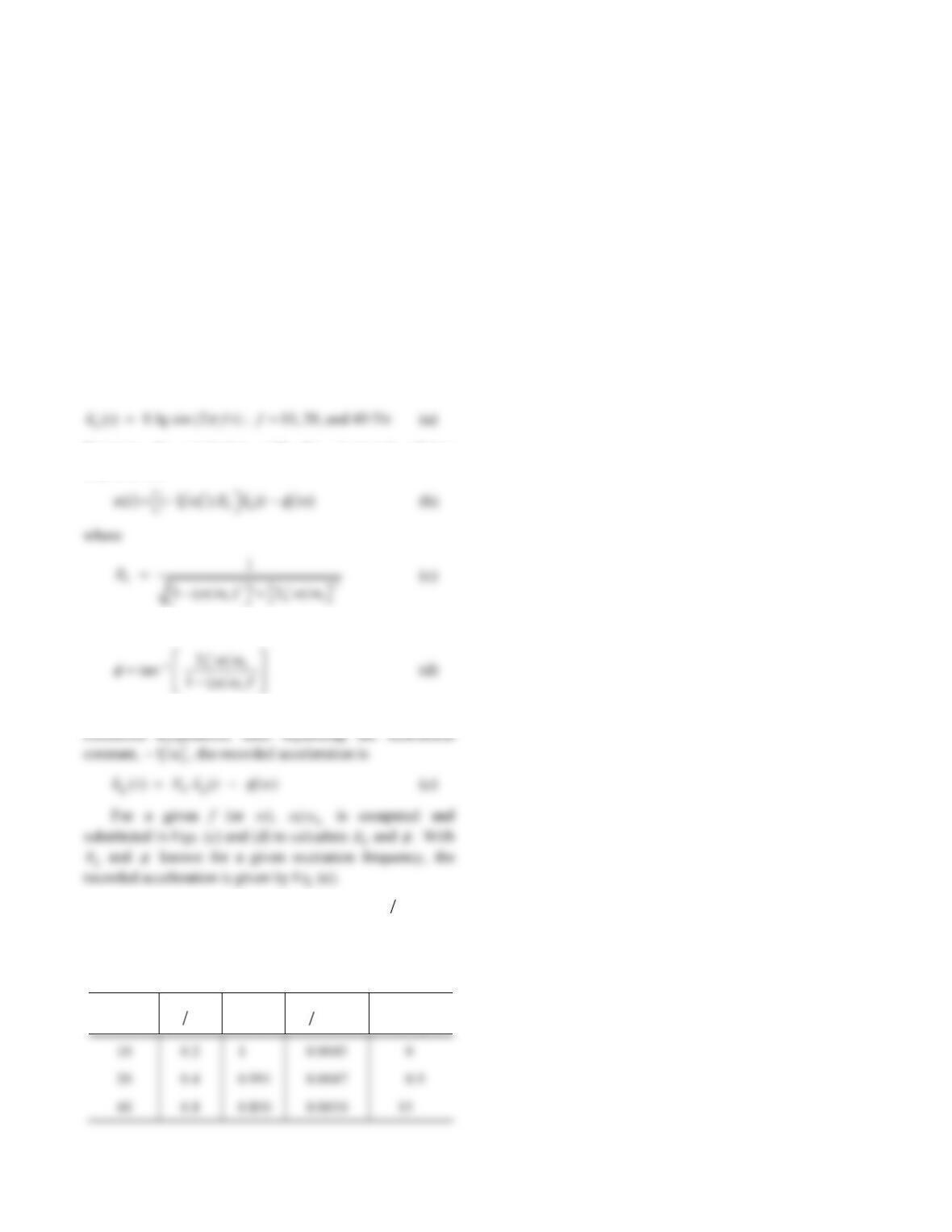
The natural frequency of an accelerometer is 50 Hz, and its
damping ratio is 70%. Compute the recorded acceleration
as a function of time if the input acceleration is ug(t) = 0.1g
sin 2 πft for f = 10, 20, and 40 Hz. A comparison of the
input and recorded accelerations was presented in Fig.
3.7.3. The accelerometer is calibrated to read the input
acceleration correctly at very low values of the excitation
frequency. What would be the error in the measured
amplitude at each of the given excitation frequencies?
Solution:
The accelerometer properties are 50 cps
n
f and
0.7
; and the excitation is
Compare the excitation with the measured relative
displacement
and
Because the instrument has been calibrated at low
The computed amplitude Rd and time lag
agrees
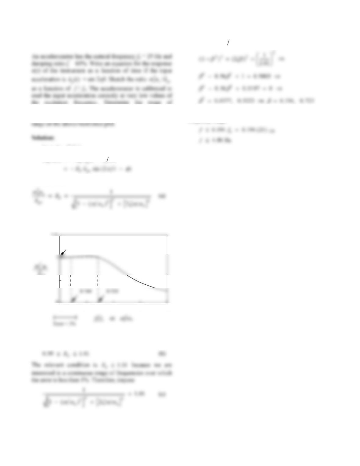
with Fig. 3.7.3. The difference between Rd and 1 is the
error in measured acceleration (Table P3.17).
Table P3.17
f
(Hz)
n Rd
, sec % error
in Rd
18
Problem 3.18
frequencies for which the acceleration amplitude can be
measured with an accuracy of ±1%. Identify this frequency
From Eq. (3.7.1),
ut R u t
2
() ()
and therefore,
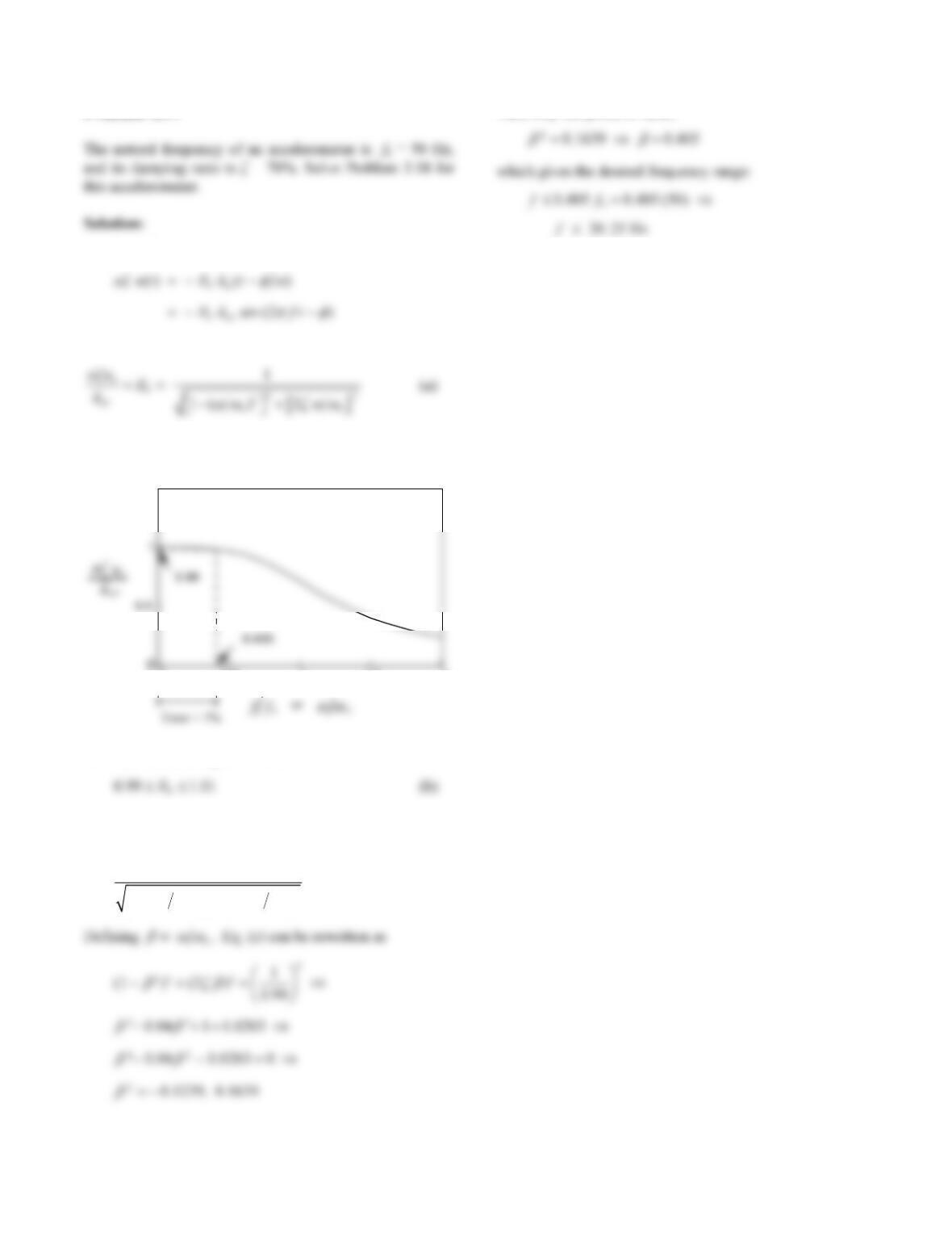
Equation (a) is plotted for
06., the accelerometer
damping ratio:
0 0.5 1 1.5 2
0.5
go
u
1.01
We want to bound Rd as follows:
Defining
n, Eq. (c) can be rewritten as
Choose
0 194. (see figure) which gives the desired
frequency range:
19
Problem 3.19
From Eq. (3.7.1),
and therefore,
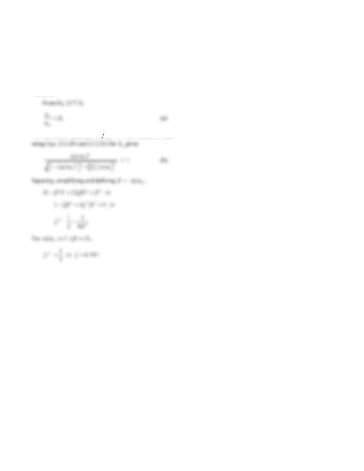
Equation (a) is plotted for 0.7
, the accelerometer
damping ratio:
0 0.5 1 1.5 2
1.5
We want to bound Rd as follows
The relevant condition is 0.99 d
R because Rd is always
smaller than 1.01 in this case. Therefore, impose
2
22
10.99
1( ) 2
nn
(c)
Take only the positive value:
20
Problem 3.20
If a displacement-measuring instrument is used to
determine amplitudes of vibration at frequencies very
much higher than its own natural frequency, what would be
the optimum instrument damping for maximum accuracy?
Solution:
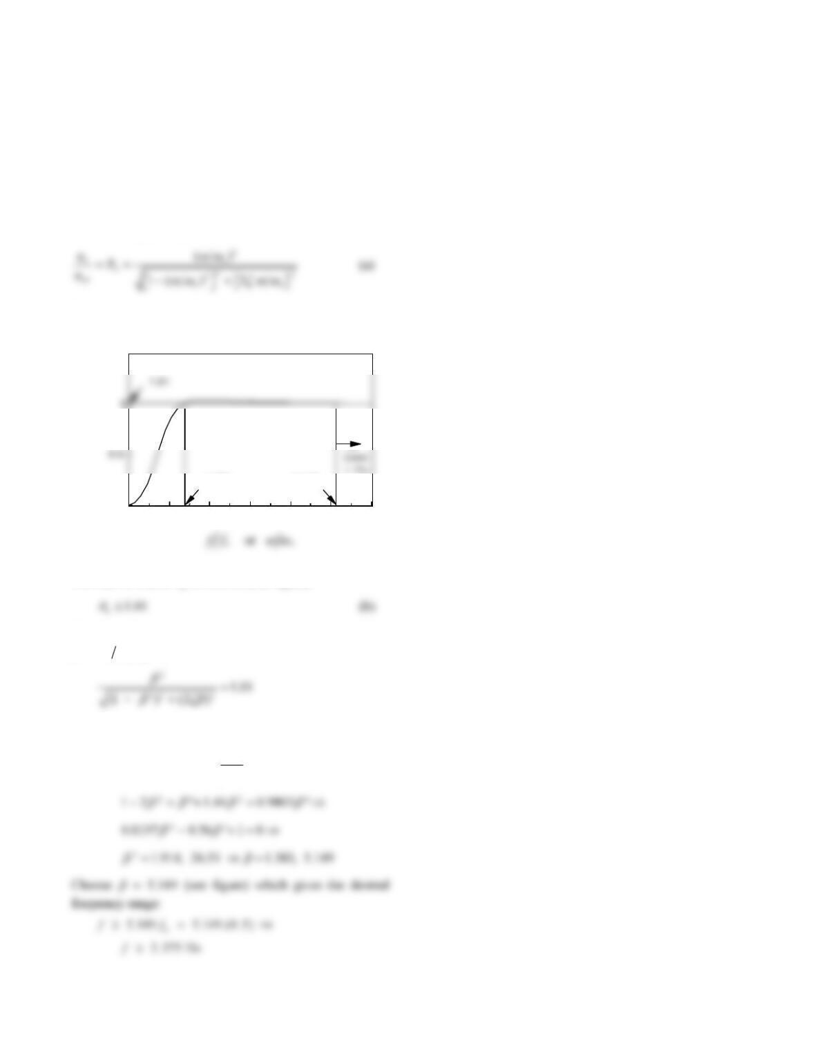
For maximum accuracy, 1
uu ; this condition after
21
Problem 3.21
A displacement meter has a natural frequency fn = 0.5 Hz
and a damping ratio ζ = 0.6. Determine the range of
frequencies for which the displacement amplitude can be
measured with an accuracy of ±1%.
Solution:
From Eq. (3.7.3),
Equation (a) is plotted for 0.6
, the instrument damping
ratio:
0 1 2 3 4 5 6
0
1.5
1.383 5.149
a
R
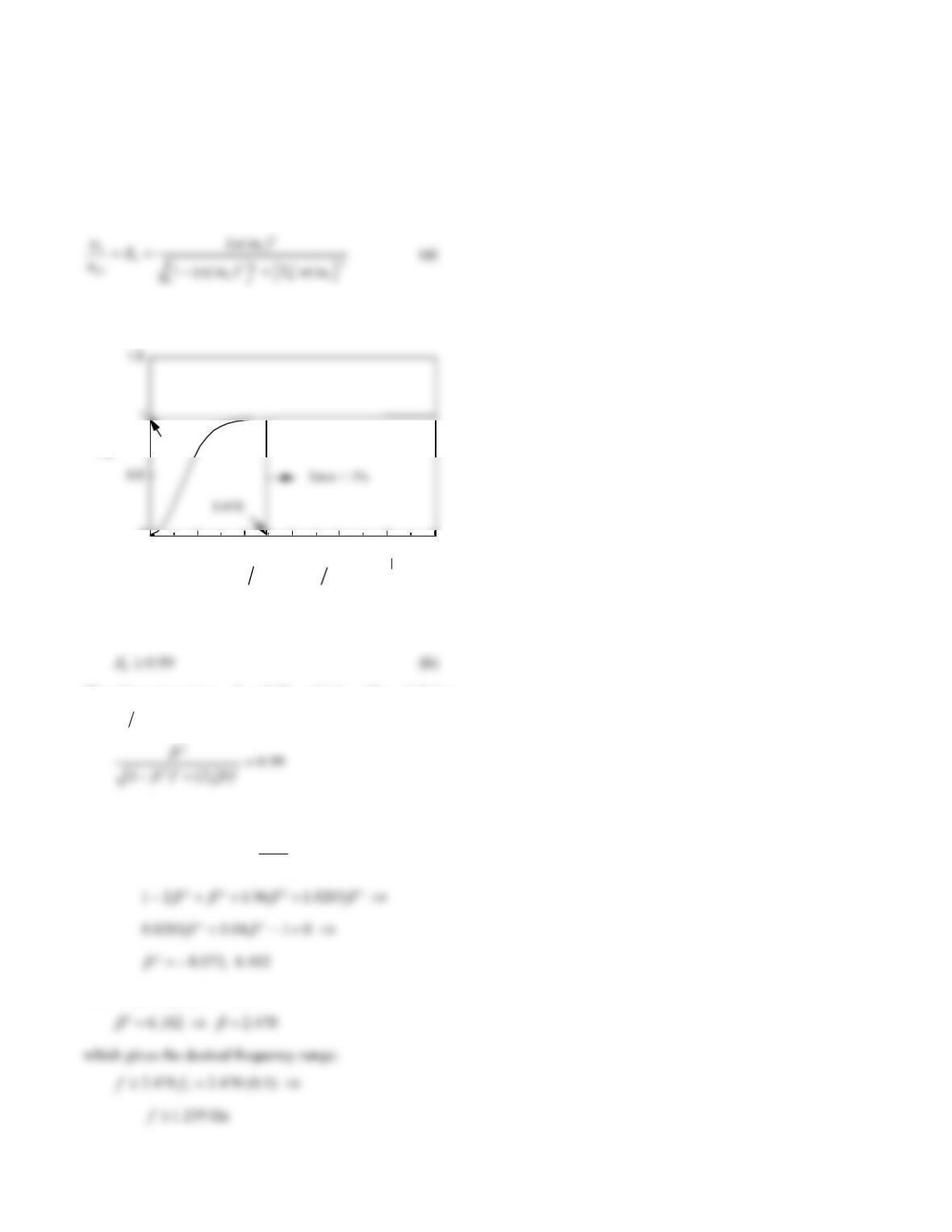
We want to bound Ra as follows (see figure)
Therefore imposing Ra101. which, after defining
n, gives
Squaring this equation gives
2
2
22 2
(1 ) ( 2 ) 1.01
22
Problem 3.22
Repeat Problem 3.21 for ζ = 0.7.
Solution:
From Eq. (3.7.3),
Equation (a) is plotted for 0.7
, the instrument damping
ratio:
0 1 2 3 4 5 6
0
0.99
f f
n n
or
a
R
Since Ra is always smaller than 1.01, we want to bound Ra
as follows
Therefore imposing 0.99
a
R which, after defining
n
, gives
Squaring this equation gives
2
2
22 2
(1 ) (2 ) 0.99
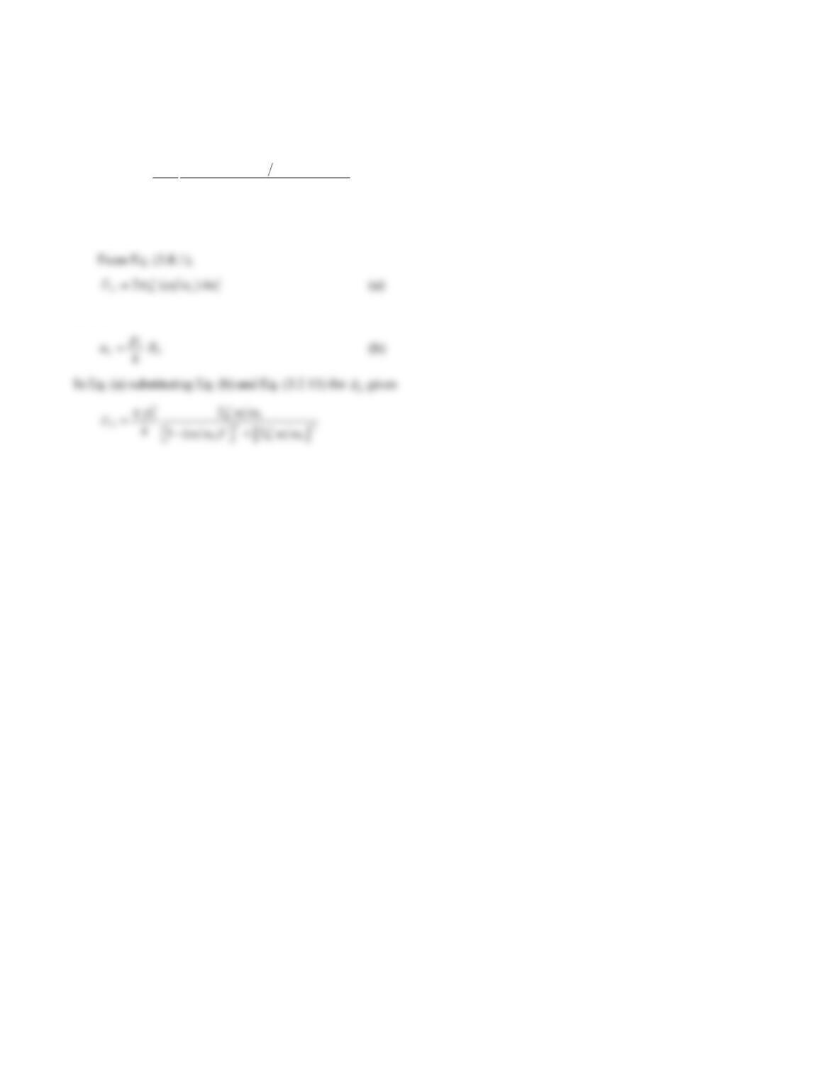
Take only the positive value:
23
Problem 3.23
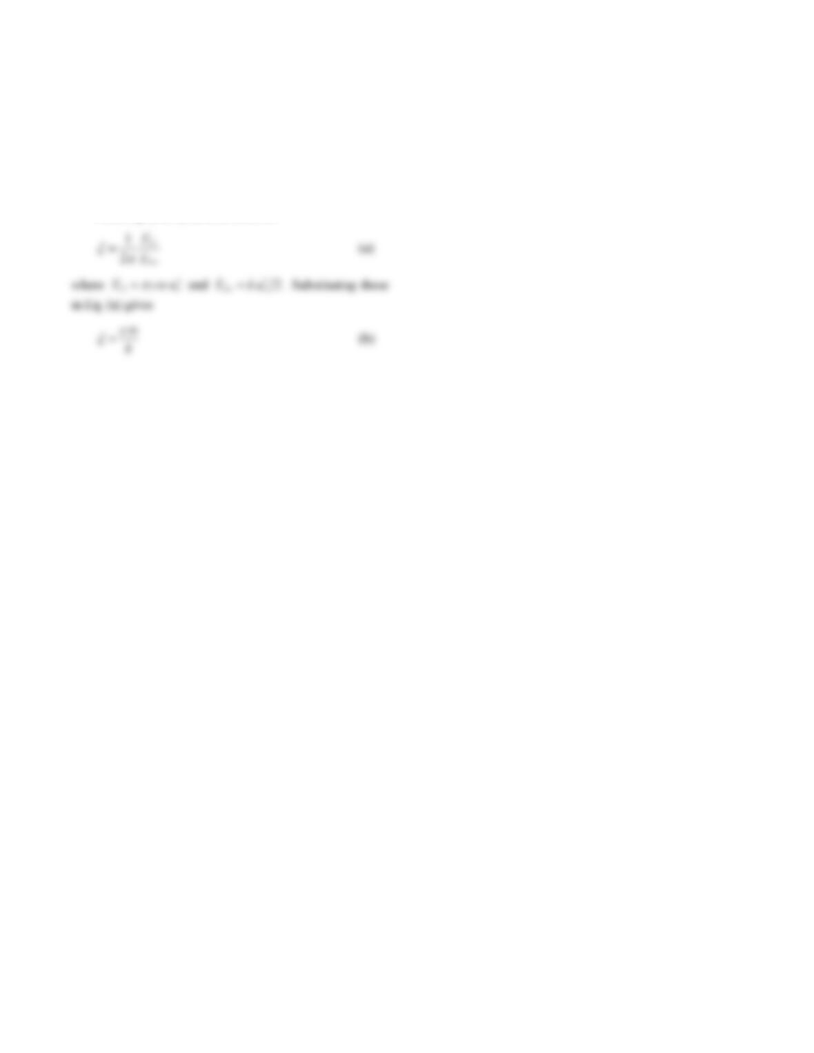
Show that the energy dissipated per cycle for viscous
damping can be expressed by
2
22
2
2( )
1(/ ) 2(/ )
on
D
nn
p
Ek
Solution:
where
24
Problem 3.24
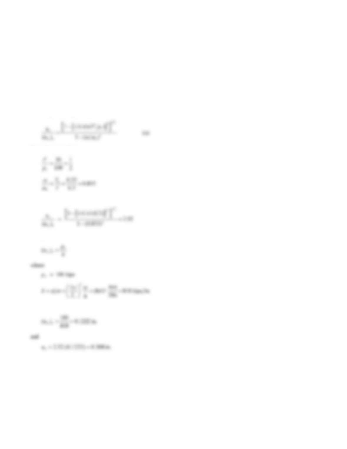
Show that for viscous damping the loss factor ξ is inde-
pendent of the amplitude and proportional to the
frequency.
Solution:
From Eq. (3.8.9) the loss factor is
25
Problem 3.25
The properties of the SDF system of Fig. P2.20 are as
follows: w = 500 kips, F = 50 kips, and Tn = 0.25 sec.
Determine an approximate value for the displacement
amplitude due to harmonic force with amplitude 100 kips
and period 0.30 sec.
Solution:
Based on equivalent viscous damping, the displace-
ment amplitude is given by
From the given data
Substituting these data in Eq. (a) gives
Now,
Thus
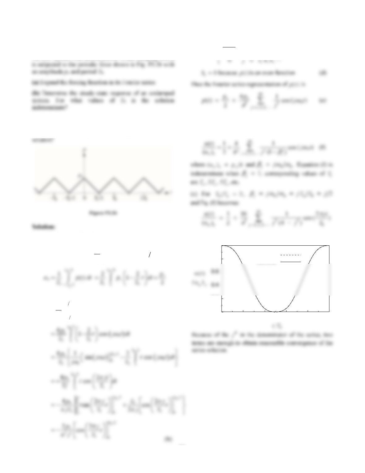
26
Problem 3.26
An SDF system with natural period Tn and damping ratio ζ
(c) For T0/Tn = 2, determine and plot the response to indi-
vidual terms in the Fourier series. How many terms are
necessary to obtain reasonable convergence of the series
(a) p
t
()
is an even function:
0
2
() 1
o
pt p t
T
02
0
tT
(a)
22
41, 3, 5,
o
j
pj
j
a
(c)
(b) The steady-state response of an undamped system is
obtained by substituting Eqs. (b), (c), and (d) in Eq.
(3.13.6) to obtain
0 0.2 0.4 0.6 0.8 1
0
0.2
0.8
1
two terms
three terms
2
0
02
0
0
2cos
T
j
T
aptjtdt
T