Iterative Methods, Basic Concepts 1
3.8 Iterative Methods, Basic Concepts
In Exercises 1 – 4:
(a) Compute Tjac and Tgs for the given matrix.
(b) Determine the spectral radius of each iteration matrix from part (a).
(c) Will the Jacobi method converge for any choice of initial vector x(0)? Will
the Gauss-Seidel method converge for any choice of initial vector x(0)? Explain.
1. 2−1
−1 3
Let
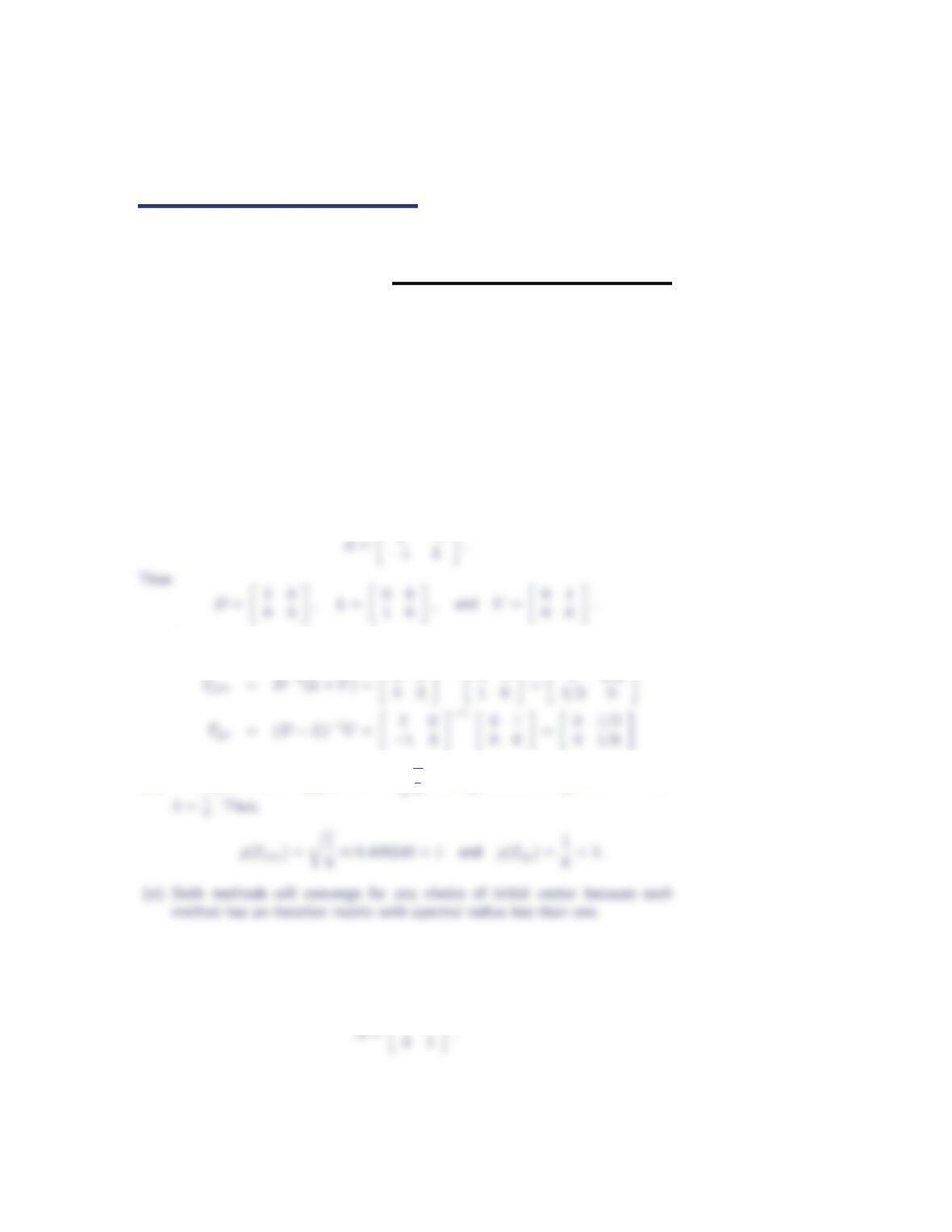
(a) The iteration matrices are
(b) The eigenvalues of Tjac are λ=±q1
6; the eigenvalues of Tgs are λ= 0 and
2. 1 2
3 4
Let
2Section 3.8
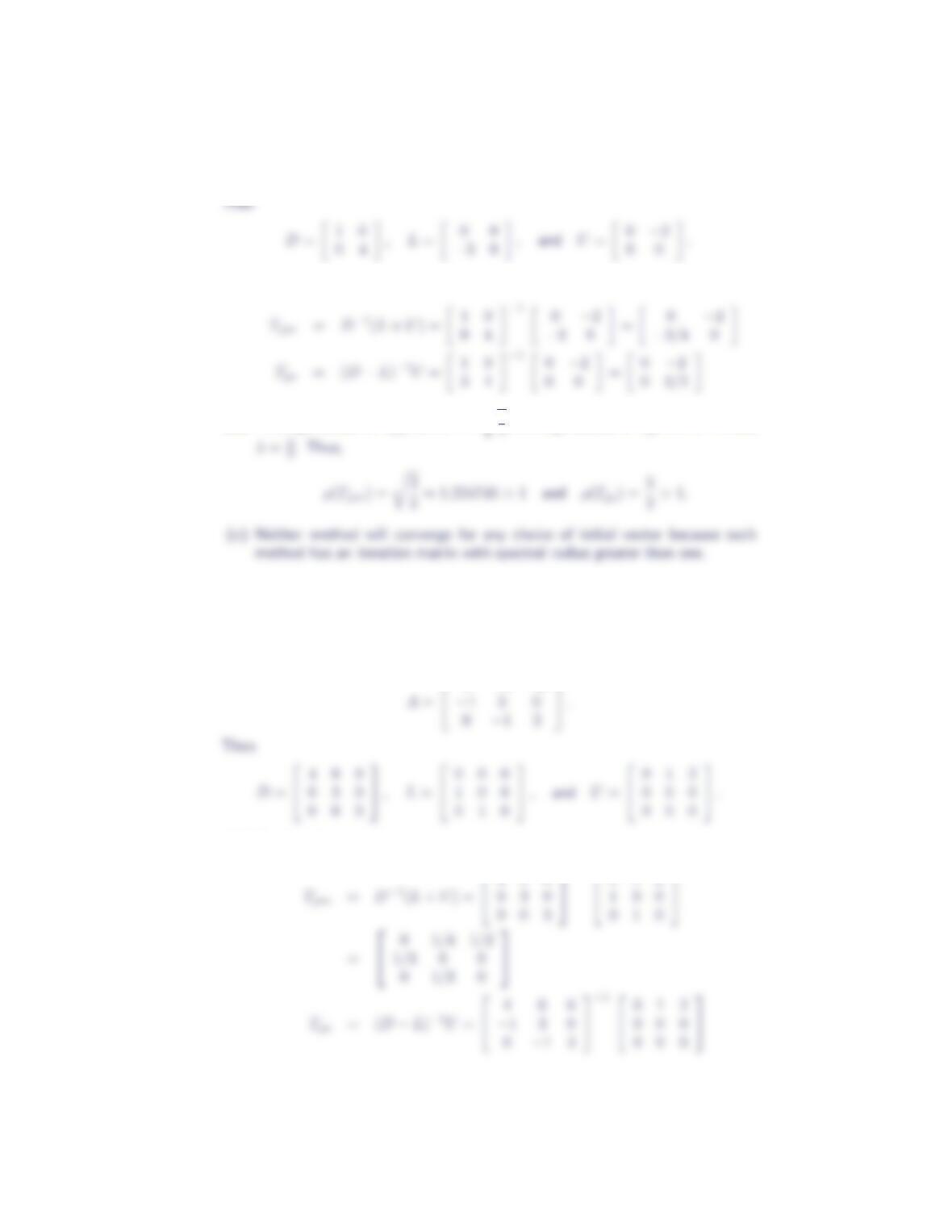
(a) The iteration matrices are
(b) The eigenvalues of Tjac are λ=±q3
3.
4−1−2
−1 3 0
0−1 3
Let
4−1−2
(a) The iteration matrices are
400
−1
012
Iterative Methods, Basic Concepts 3
0 1/4 1/2
4.
3 2 −2
−2−2 1
5−5 4
Let
3 2 −2
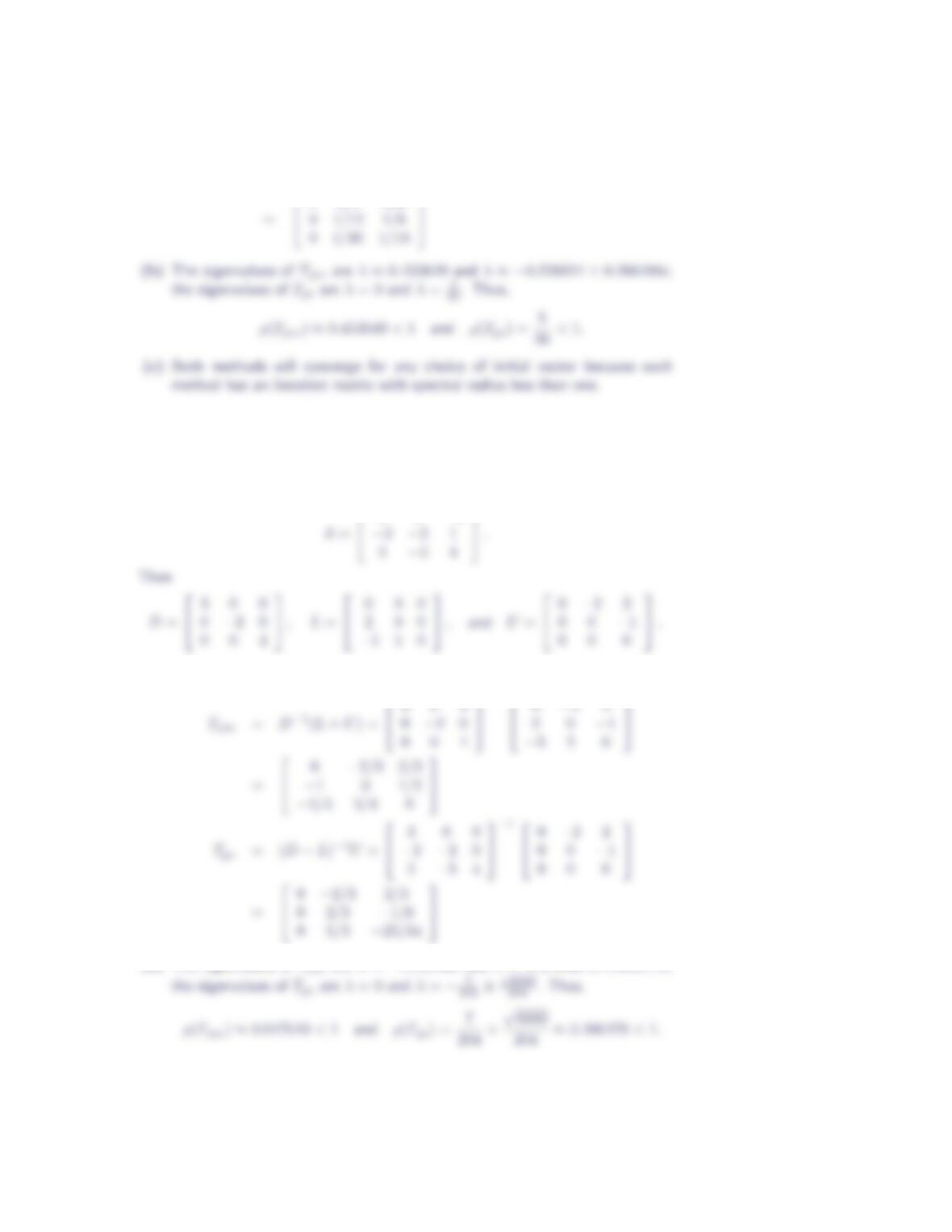
(a) The iteration matrices are
−1
(b) The eigenvalues of Tjac are λ≈ −0.947640 and λ≈0.473820 ±0.463878i;
4Section 3.8
5. For each of the following coefficient matrices and right-hand side vectors, write
out the components of the Jacobi method iteration equation. Then, starting
with the initial vector x(0) =0, perform two iterations of the Jacobi method.
(a)
2−1 0
−142
0 2 6
,
−1
3
5
(b)
3−1 1
2−6 3
−9 7 −20
,
4
−13
7
(c)
4 2 −1
241
−1 1 4
,
1
−1
1
(d)
4−1 0 0
2 4 −1 0
0−2 4 −1
0 0 −2 4
,
0
2
−3
1
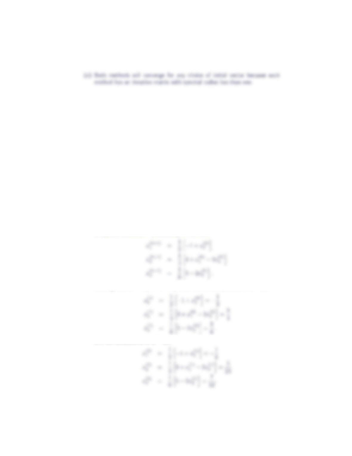
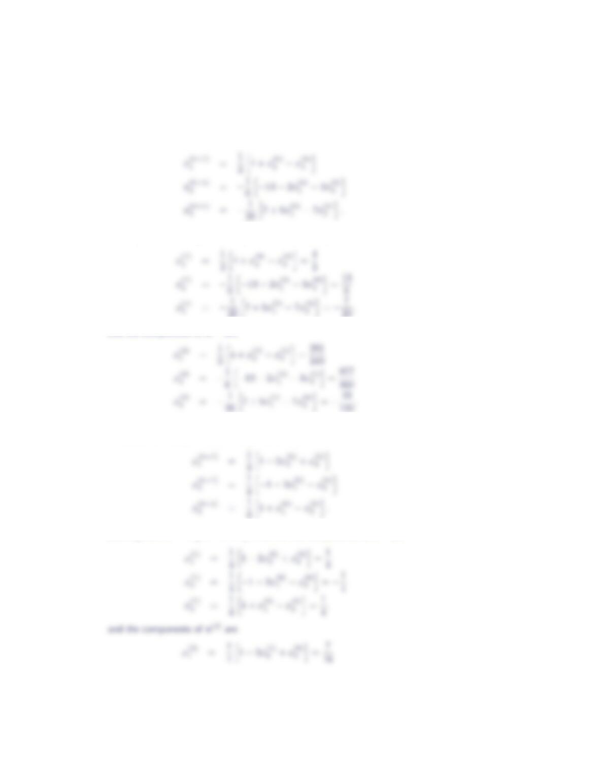
(a) The Jacobi method, when applied to this system, will produce the sequence
of approximations {x(k)}according to the rules
Starting from x(0) =000T, we find the components of x(1) are
and the components of x(2) are
Iterative Methods, Basic Concepts 5
(b) The Jacobi method, when applied to this system, will produce the sequence
of approximations {x(k)}according to the rules
Starting from x(0) =000T, we find the components of x(1) are
20 h7 + 9x(0)
20.
and the components of x(2) are
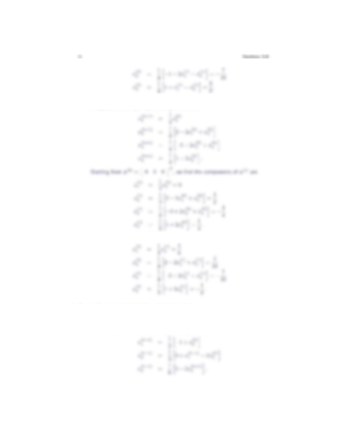
(c) The Jacobi method, when applied to this system, will produce the sequence
of approximations {x(k)}according to the rules
Starting from x(0) =000T, we find the components of x(1) are
(d) The Jacobi method, when applied to this system, will produce the sequence
of approximations {x(k)}according to the rules
and the components of x(2) are
6. Repeat Exercise 5 for the Gauss-Seidel method.
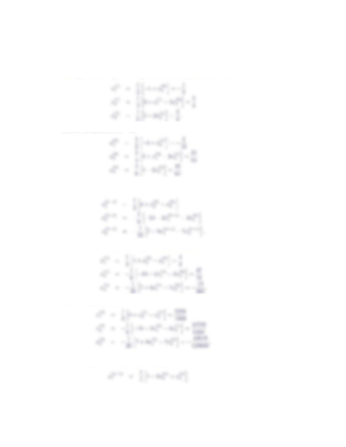
(a) The Gauss-Seidel method, when applied to this system, will produce the se-
quence of approximations {x(k)}according to the rules
Iterative Methods, Basic Concepts 7
Starting from x(0) =000T, we find the components of x(1) are
and the components of x(2) are
(b) The Gauss-Seidel method, when applied to this system, will produce the se-
quence of approximations {x(k)}according to the rules
Starting from x(0) =000T, we find the components of x(1) are
and the components of x(2) are
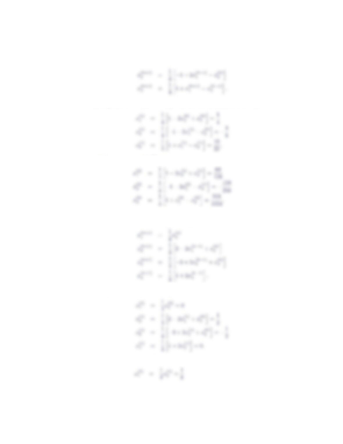
(c) The Gauss-Seidel method, when applied to this system, will produce the se-
quence of approximations {x(k)}according to the rules
8Section 3.8
Starting from x(0) =000T, we find the components of x(1) are
and the components of x(2) are
(d) The Gauss-Seidel method, when applied to this system, will produce the se-
quence of approximations {x(k)}according to the rules
Starting from x(0) =000T, we find the components of x(1) are
and the components of x(2) are
Iterative Methods, Basic Concepts 9
In Exercises 7 – 10, use both the Jacobi method and the Gauss-Seidel method
to solve the indicated linear system of equations. Take x(0) =0, and terminate
iteration when kx(k+1) −x(k)k∞falls below 5 ×10⁻⁶. Record the number of
iterations required to achieve convergence.
7.
4x1+x2+x3+x4=−5
x1+ 8x2+ 2x3+ 3x4= 23
x1+ 2x2−5x3= 9
−x1+ 2x3+ 4x4= 4
26 iterations of the Jacobi method are needed to produce the solution vector
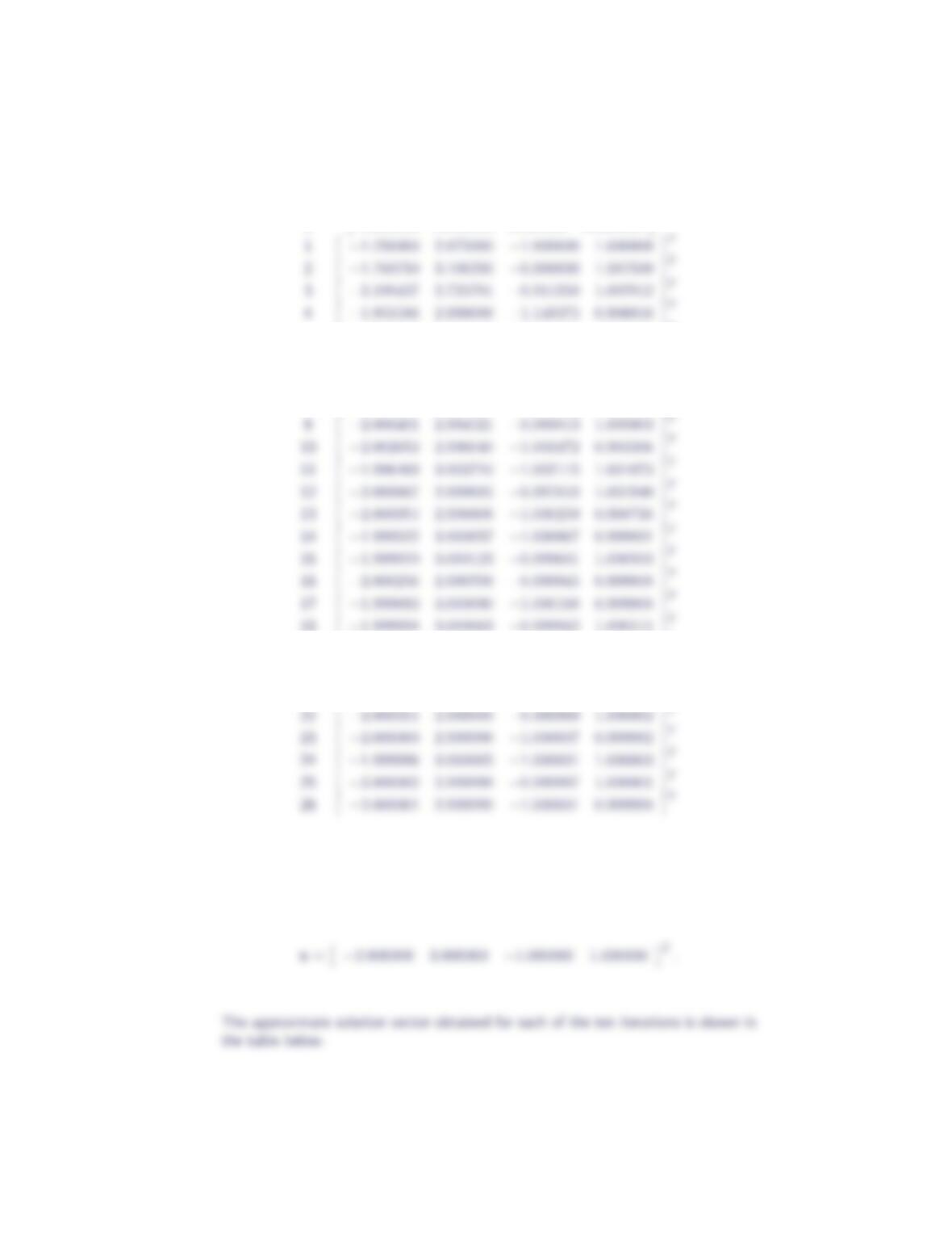
10 Section 3.8
kx(k)
00.000000 0.000000 0.000000 0.000000 T
5−1.939082 3.067036 −0.991242 1.085791 T
6−2.040396 2.958024 −0.961002 1.010851 T
7−2.001968 2.991231 −1.024870 0.970402 T
8−1.984191 3.017563 −1.003901 1.011943 T
19 −2.000058 2.999939 −0.999966 0.999982 T
20 −1.999989 3.000006 −1.000036 0.999969 T
21 −1.999985 3.000019 −0.999995 1.000021 T
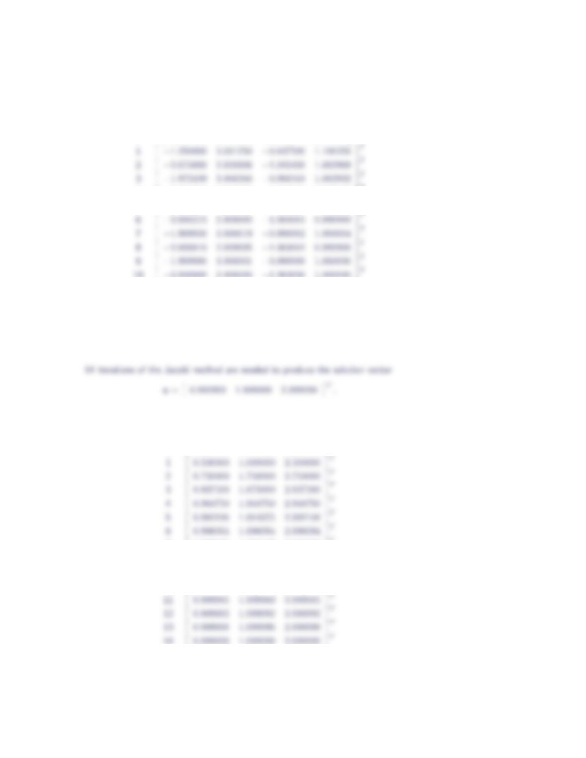
Ten iterations of the Gauss-Seidel method are needed to produce the solution vector
Iterative Methods, Basic Concepts 11
kx(k)
00.000000 0.000000 0.000000 0.000000 T
4−2.004318 2.997420 −1.001896 0.999868 T
5−1.998848 3.000379 −0.999618 1.000097 T
8.
4x1−x2= 2
−x1+ 4x2−x3= 4
−x2+ 4x3= 10
The approximate solution vector obtained for each of the 14 iterations is shown in
the table below.
kx(k)
00.000000 0.000000 0.000000 T
70.999023 1.998047 2.999023 T
80.999512 1.999512 2.999512 T
90.999878 1.999756 2.999878 T
10 0.999939 1.999939 2.999939 T
12 Section 3.8
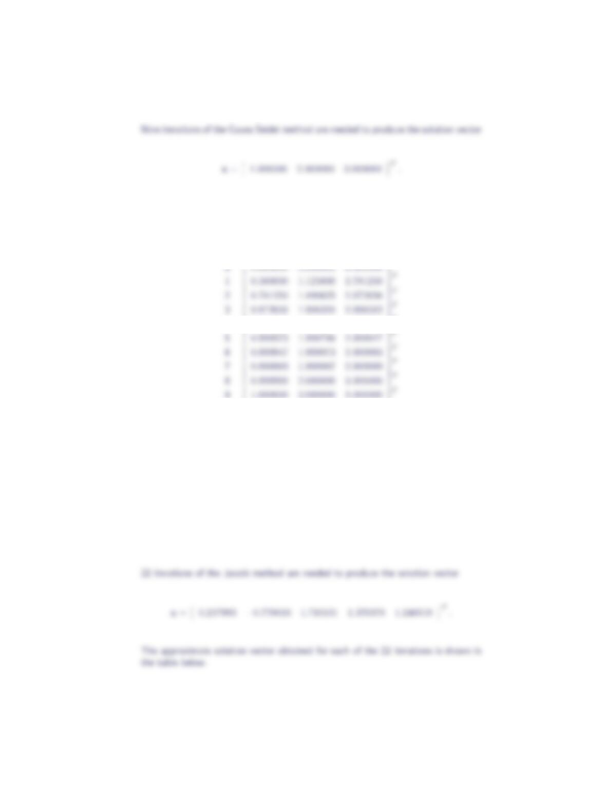
The approximate solution vector obtained for each of the nine iterations is shown
in the table below.
kx(k)
40.996582 1.998291 2.999573 T
9.
7x1−3x2= 4
−3x1+ 9x2+x3=−6
x2+ 3x3−x4= 3
−x3+ 10x4−4x5= 7
−4x4+ 6x5= 2