3.4 Error Estimates and Condition Number
1. Let Aand Bbe n×nmatrices, and let αbe a non-zero real number.
(a) Show that κ(AB)≤κ(A)κ(B).
(b) Show that κ(αA) = κ(A).
(a)
2. Let Abe an n×nmatrix, and suppose that Ax=yfor some vectors xand y.
Show that
κ(A)≥kAkkxk
kyk.
3. (a) Let Abe a nonsingular matrix. Show that if
kA−Bk<1/kA−1k,
then Bis nonsingular. (Hint: Write B=A−(A−B) = A(I−A−1(A−B)),
and focus on the matrix A−1(A−B). You will need to use Exercise 10
from Section 3.3.)
2Section 3.4
(b) Let Abe a nonsingular matrix and suppose that kδAk<1/kA−1k. Show
that A+δA is nonsingular.
(a) Following the hint, write B=A−(A−B) = A(I−A−1(A−B)). Because
(b) Let B=A+δA. Then
4. For each of the following floating point number systems, what is roughly the
largest condition number for which the solution to the system Ax=b, computed
in that number system using Gaussian elimination with pivoting, would be
accurate to ten (10) decimal digits? See Section 1-3 for an explanation of the
notation.
(a) IEEE standard double precision, F(2,53,−1021,1024)
(b) Intel extended precision, F(2,64,−16381,16384)
(c) HP double extended precision, F(2,113,−16381,16384)
(d) IBM System/390 long precision, F(16,14,−64,63)
(e) IBM System/390 extended precision, F(16,28,−64,63)
(a) Machine precision for F(2,53,−1021,1024) is
Error Estimates and Condition Number 3
(c) Machine precision for F(2,113,−16381,16384) is
(d) Machine precision for F(16,14,−64,63) is
(e) Machine precision for F(16,28,−64,63) is
5. Suppose the matrix Ahas a condition number of ≈105. If the system of
equations Ax=bis solved using Gaussian elimination with pivoting in each
of the following floating point number systems, how many decimal digits of
precision can be expected in the approximate solution?
(a) IEEE standard double precision, F(2,53,−1021,1024)
(b) Intel extended precision, F(2,64,−16381,16384)
(c) HP double extended precision, F(2,113,−16381,16384)
(d) IBM System/390 long precision, F(16,14,−64,63)
(e) IBM System/390 extended precision, F(16,28,−64,63)
(f) IEEE standard single precision, F(2,24,−125,128)
(g) IBM System/390 short precision, F(16,6,−64,63)
4Section 3.4
(a) Machine precision for F(2,53,−1021,1024) is
(b) Machine precision for F(2,64,−16381,16384) is
(c) Machine precision for F(2,113,−16381,16384) is
(d) Machine precision for F(16,14,−64,63) is
(e) Machine precision for F(16,28,−64,63) is
(f) Machine precision for F(2,24,−125,128) is
Error Estimates and Condition Number 5
6. Repeat Exercise 5 if the matrix Ahas a condition number of ≈1012.
(a) Machine precision for F(2,53,−1021,1024) is
(b) Machine precision for F(2,64,−16381,16384) is
(c) Machine precision for F(2,113,−16381,16384) is
(d) Machine precision for F(16,14,−64,63) is
6Section 3.4
leaving between 3 and 4 decimal digits of precision in the approximate solution.
(e) Machine precision for F(16,28,−64,63) is
(f) Machine precision for F(2,24,−125,128) is
(g) Machine precision for F(16,6,−64,63) is
7. Compute κ∞for each of the following matrices.
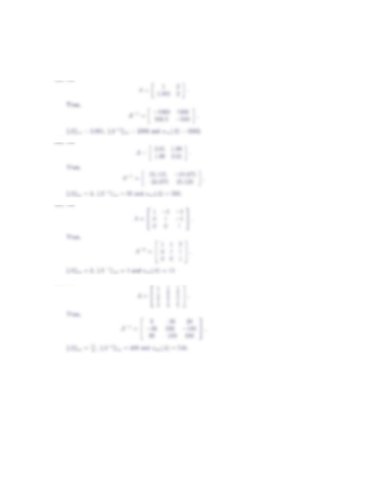
(a) A=1 2
1.001 2
(b) A=2.01 1.99
1.99 2.01
(c) A=
1−1−1
0 1 −1
0 0 1
(d) A=
11
2
1
3
1
2
1
3
1
4
1
3
1
4
1
5
Error Estimates and Condition Number 7
(d) Let
8. In each of the following problems, a linear system Ax=bis given, along with
the exact solution, x, and an approximate solution, ˜
x. Compute the error
e=˜
x−xand the residual r=A˜
x−band then compare the relative error to
the condition number times the relative residual. Use the l∞norm in all cases.
Note that the coefficient matrices in these problems are the same matrices from
Exercise 7.
8Section 3.4
(a) 1 2
1.001 2 x=3
3.001
x=1 1 T
˜
x=3 0 T
(b) 2.01 1.99
1.99 2.01 x=4
4
x=1 1 T
˜
x=2 0 T
(c)
1−1−1
0 1 −1
0 0 1
x=
0
2
0
x=220T
˜
x=1.9 2.1−0.1T
(d)
11
2
1
3
1
2
1
3
1
4
1
3
1
4
1
5
x=
1
7
12
13
30
x=1−2 3 T
˜
x=1.02 −1.96 2.94 T
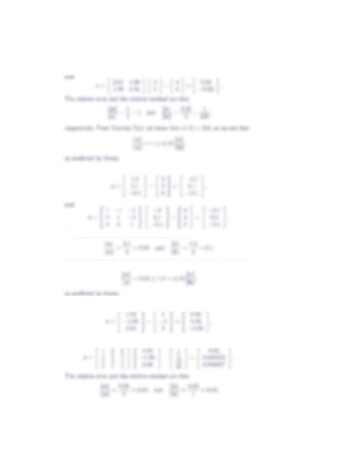
(a) First, we calculate
The relative error and the relative residual are then
(b) First, we calculate
Error Estimates and Condition Number 9
(c) First, we calculate
The relative error and the relative residual are then
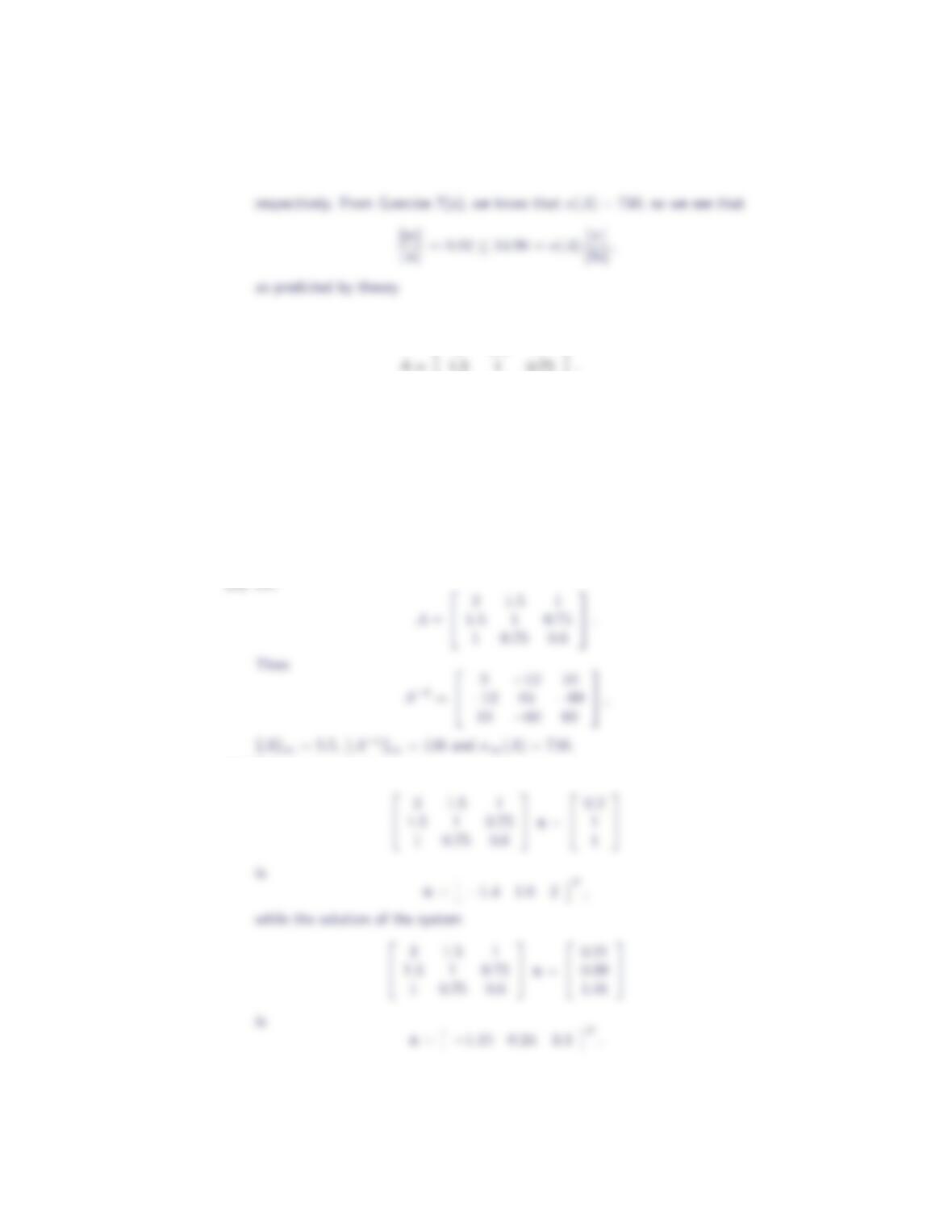
respectively. From Exercise 7(a), we know that κ(A) = 12, so we see that
(d) First, we calculate
and
10 Section 3.4
9. Let
3 1.5 1
1 0.75 0.6
(a) Compute κ∞(A).
(b) Let b=0.211T, and solve the system Ax=b. Now perturb bby
δb=0.01 −0.01 0.01 Tand solve the resulting perturbed system.
Compare the actual value of kδxk∞/kxk∞with the theoretical upper
bound predicted by equation (5).
(c) Repeat part (b), but start with b=5.5 3.25 2.35 T.
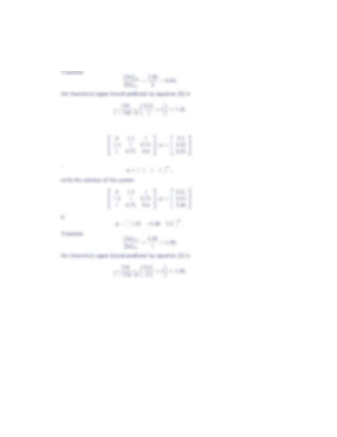
(a) Let
(b) The solution of the system
Error Estimates and Condition Number 11
(c) The solution of the system
is
10. Let
A=25 19
21 16 .
(a) Compute κ∞(A).
(b) Let b=6 5 T, and solve the system Ax=b. Now perturb bby
δb=0.01 −0.01 Tand solve the resulting perturbed system. Com-
pare the actual value of kδxk∞/kxk∞with the theoretical upper bound
predicted by equation (5).
(c) Repeat part (b), but start with b=1 1 T.
12 Section 3.4
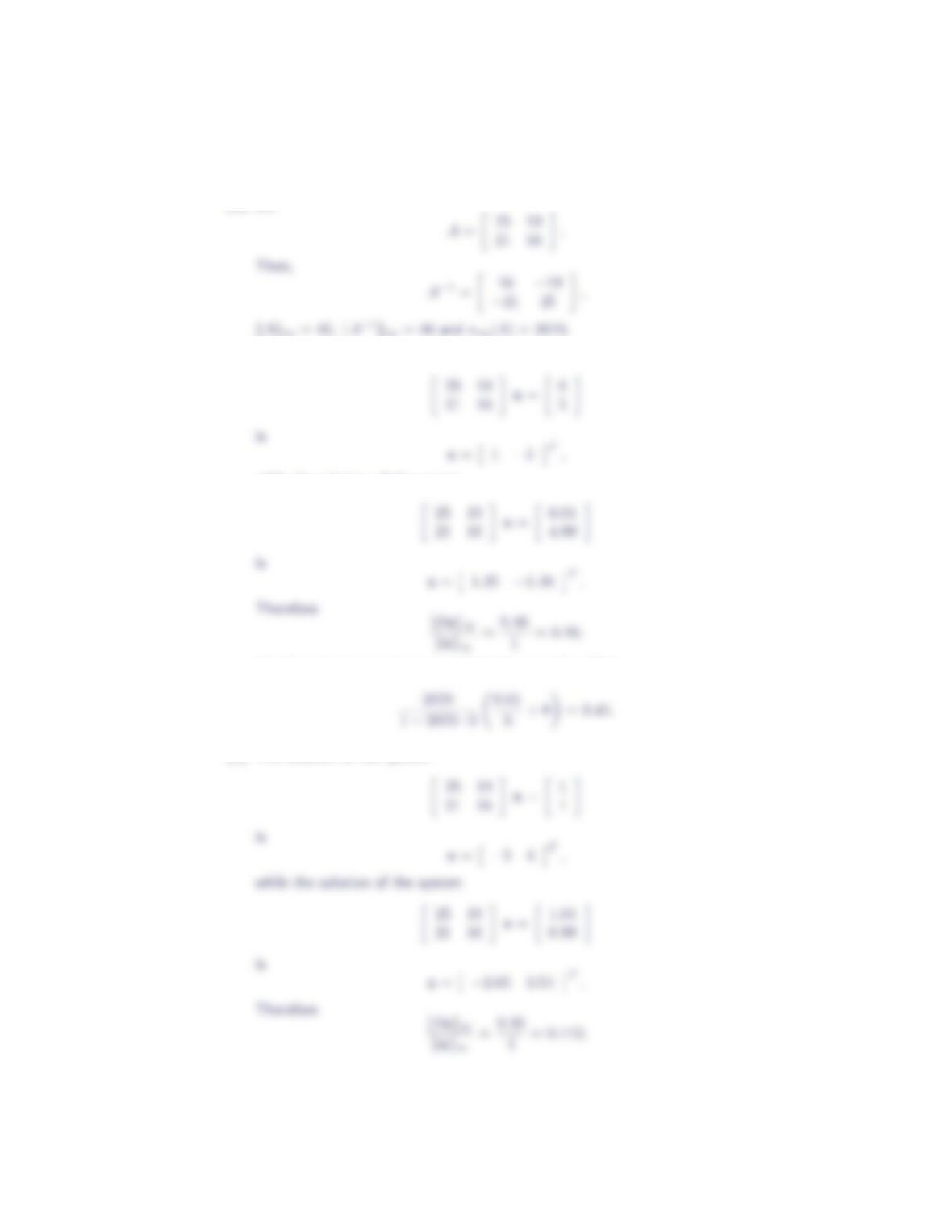
(a) Let
(b) The solution of the system
while the solution of the system
the theoretical upper bound predicted by equation (5) is
(c) The solution of the system
Error Estimates and Condition Number 13
the theoretical upper bound predicted by equation (5) is
11. Let
A=
0.25 0.35 0.15
0.20 0.20 0.25
0.15 0.20 0.25
and b=
0.60
0.90
0.70
.
(a) Compute κ∞(A).
(b) Solve the system Ax=b.
(c) Perturb the coefficient matrix and right-side vector by
δA =
0.01 0 0
0 0 −0.01
0−0.01 0
and δb=
0.01
0.02
−0.03
and solve the resulting perturbed system. Compare the actual value of
kδxk∞/kxk∞with the theoretical upper bound predicted by equation (5).
(d) Perturb the original coefficient matrix and right-side vector by
δA =
0−0.01 0.01
−0.01 0.01 0
0.01 0 0.01
and δb=
0.02
0.01
−0.01
and solve the resulting perturbed system. Compare the actual value of
kδxk∞/kxk∞with the theoretical upper bound predicted by equation (5).
(a) Let
(b) The solution of the system
14 Section 3.4
(c) The solution of the system
(d) The solution of the system
12. Let
A=5.1 8.7
2.4 4.1and b=9.48
4.48 .
(a) Compute κ∞(A).
(b) Solve the system Ax=b.
(c) Perturb the coefficient matrix and right-side vector by
δA =−0.001 0
0.001 0 and δb=0.05
−0.05
and solve the resulting perturbed system. Compare the actual value of
kδxk∞/kxk∞with the theoretical upper bound predicted by equation (5).
Error Estimates and Condition Number 15
(d) Perturb the original coefficient matrix and right-side vector by
δA =0.001 −0.001
−0.001 0.001 and δb=−0.1
0.1
and solve the resulting perturbed system. Compare the actual value of
kδxk∞/kxk∞with the theoretical upper bound predicted by equation (5).
(a) Let
(b) The solution of the system
(c) The solution of the system
(d) The solution of the system
16 Section 3.4
13. Let Abe the n×nmatrix whose entries are given by aij = 1/(i+j−1) for
1≤i, j ≤n.
(a) For n= 5, solve the system Ax=busing Gaussian elimination with
scaled partial pivoting in single precision arithmetic. Take bas the vector
that corresponds to an exact solution of xi= 1 for each i= 1,2,3, …, n.
Estimate κ(A) based on the results of this experiment.
(b) Repeat part (a) with n= 11 and double precision arithmetic.
(a) Solving the system
11
2
1
3
1
4
1
5
137
60
we see that the computed solution agrees with the exact solution to at least
(b) Solving the indicated system using Gaussian elimination with scaled partial
pivoting and double precision arithmetic, we obtain the solution vector
Error Estimates and Condition Number 17
14. Solve the following system in single precision arithmetic.
−149x1−50x2−154x3= 353
537x1+ 180x2+ 546x3=−1263
−27x1−9x2−25x3= 61
Use Gaussian elimination with scaled partial pivoting. The exact solution for
this problem is x=−1−1−1T. Estimate the condition number of the
coefficient matrix based on the outcome of this experiment.
Solving the indicated system using Gaussian elimination with scaled partial pivoting
15. Solve the following system in double precision arithmetic.
−9 11 −21 63 −252
70 −69 141 −421 1684
−575 575 −1149 3451 −13801
3891 −3891 7782 −23345 93365
1024 −1024 2048 −6144 24572
−356
2385
−19551
132274
34812
Use Gaussian elimination with scaled partial pivoting. The exact solution for
this problem is x=1−1 1 −1 1 T. Estimate the condition number of
the coefficient matrix based on the outcome of this experiment.
18 Section 3.4
Solving the indicated system using Gaussian elimination with scaled partial pivoting
and double precision arithmetic, we obtain the solution vector
x=1.00000 −0.864684 0.0850087 5.26962 2.64956 T.
The least accurate component of the solution vector is the fourth component, which
does not agree with the exact solution to any decimal digits. Because IEEE standard
double precision provides between 15 and 16 decimal digits of accuracy, we estimate
that κ(A)≥1015.