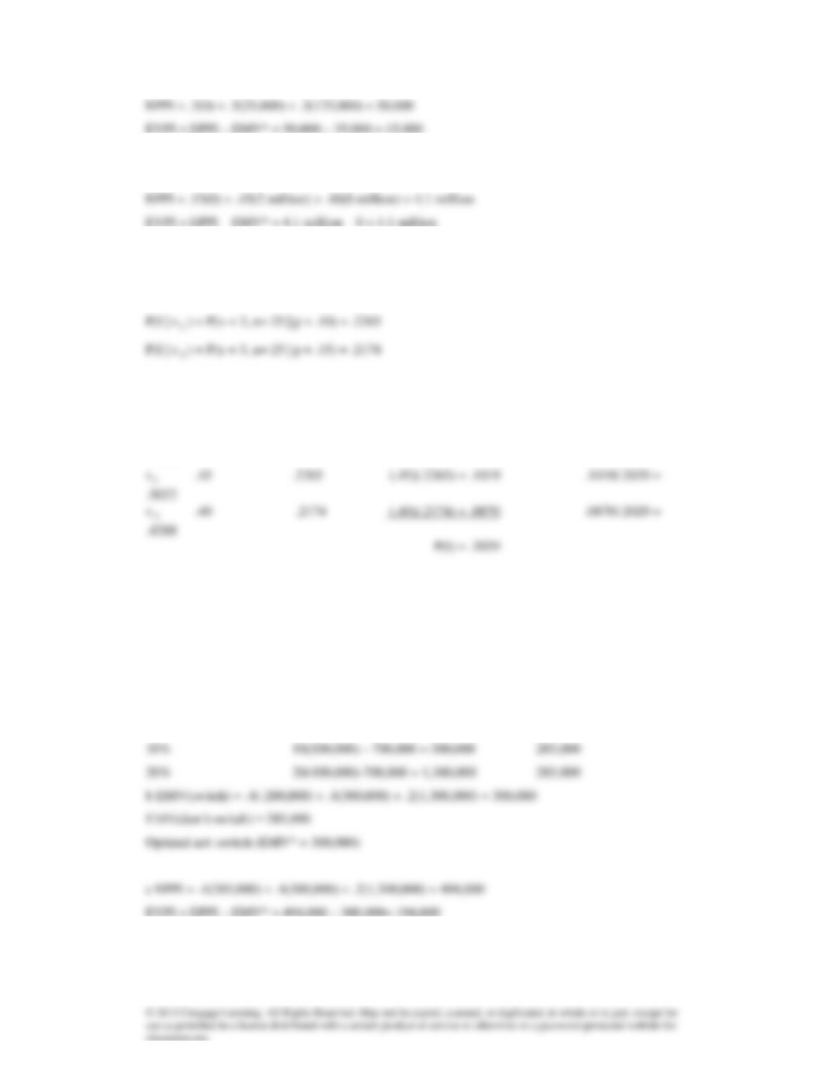
22.30 EMV* = 0
22.31 Likelihood probabilities (binomial probabilities)
P(I | s
1
) = P(x = 3, n= 25 | p = .05) = .0930
Posterior Probabilities
s
j
P(s
j
) P(I | s
j
) P(s
j
and I) P(s
j
| I)
__________________________________________________________________________
s
1
.15 .0930 (.15)(.0930) = .0140 .0140/.2029 =
.0690
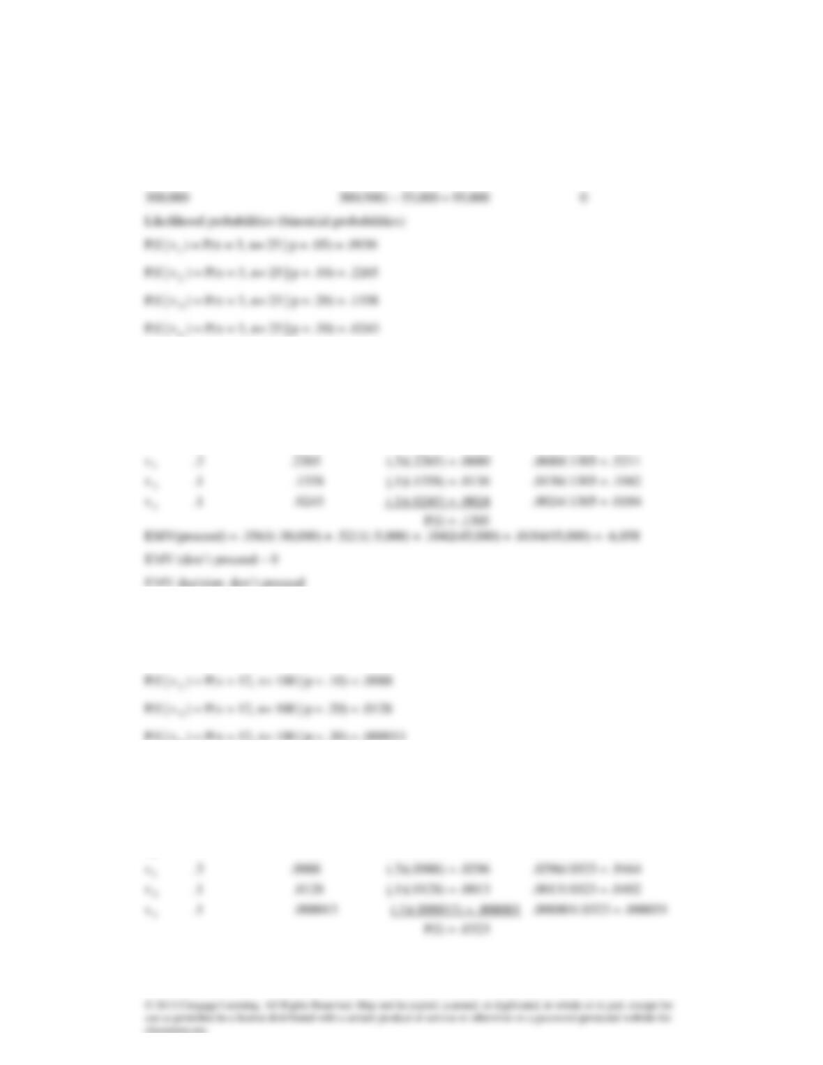
EMV(produce) = .0690(-28 million) + .5022(2 million) + .4288(8 million) = 2.503 million
EMV (don’t produce) = 0
EMV decision: produce
22.32a Payoff Table
Market share Switch Don’t switch
5% 5(100,000) – 700,000 = -200,000 285,000
22.33 Payoff Table
Participating Households Proceed Don’t proceed
50,000 50(500) – 55,000 = -30,000 0
100,000 100(500) – 55,000 = -5,000 0
200,000 200(500) – 55,000 = 45,000 0
1
2
4
Posterior Probabilities
s
j
P(s
j
) P(I | s
j
) P(s
j
and I) P(s
j
| I)
__________________________________________________________________________
s
1
. 5 .0930 (.5)(.0930) = .0465 .0465/.1305 = .3563
4
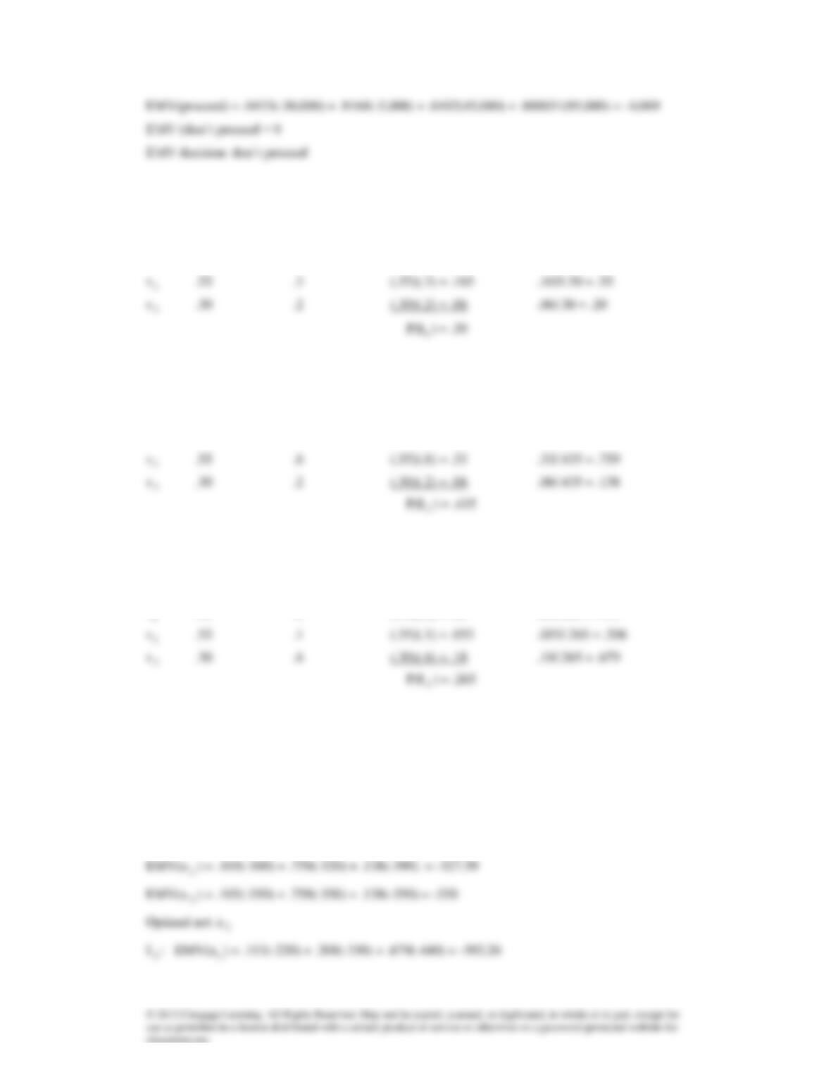
22.34 Likelihood probabilities (binomial probabilities)
P(I | s
1
) = P(x = 12, n= 100 | p = .05) = .0028
2
P(I | s
4
) = P(x = 12, n= 100 | p = .30) = .000013
Posterior Probabilities
s
j
P(s
j
) P(I | s
j
) P(s
j
and I) P(s
j
| I)
__________________________________________________________________________
s
1
. 5 .0028 (.5)(.0028) = .0014 .0014/.0323 = .0433
4
22.35 Posterior Probabilities for I
1
s
j
P(s
j
) P(I
1
|s
j
) P(s
j
and I
1
) P(s
j
| I
1
)
__________________________________________________________________________
s
1
.15 .5 (.15)(.5) = .075 .075/.30 = .25
1
Posterior Probabilities for I
2
s
j
P(s
j
) P(I
2
|s
j
) P(s
j
and I
2
) P(s
j
| I
2
)
__________________________________________________________________________
s
1
.15 .3 (.15)(.3) = .045 .045/.435 = .103
2
Posterior Probabilities for I
3
s
j
P(s
j
) P(I
3
|s
j
) P(s
j
and I
3
) P(s
j
| I
3
)
__________________________________________________________________________
s
1
3
.15 .2 (.15)(.2) = .03 .03/.265 = .113
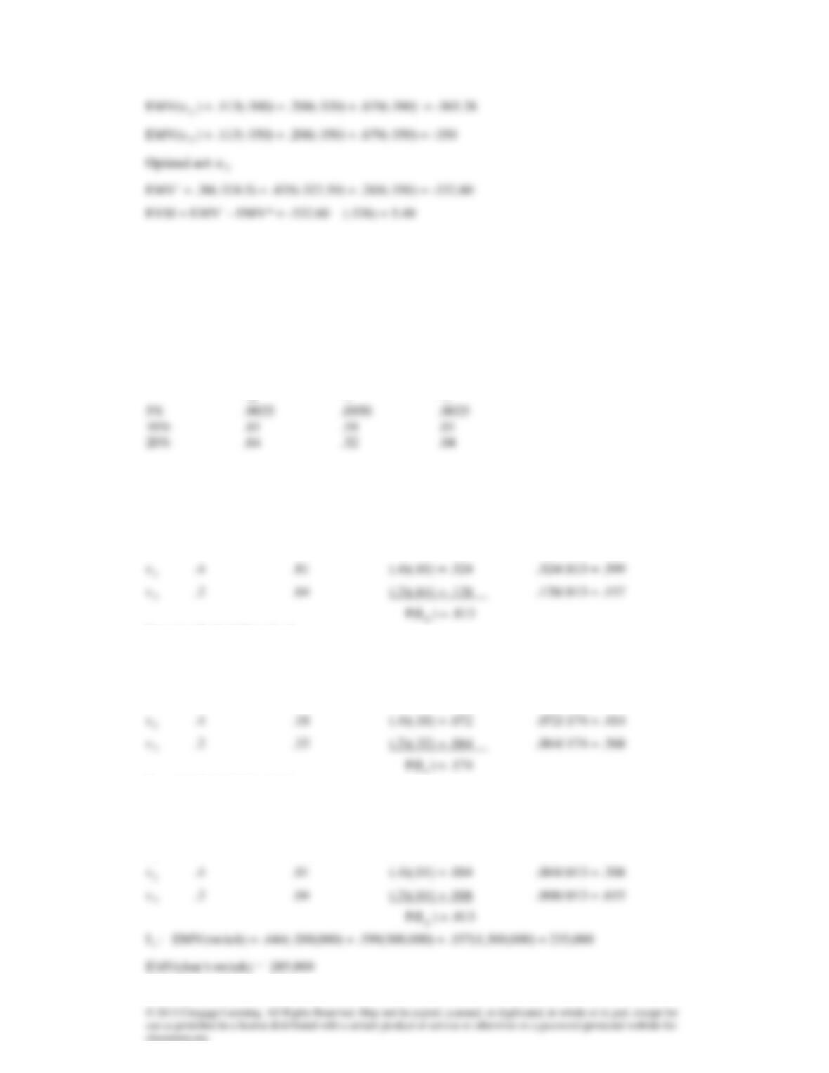
I
1
: EMV(a
1
) = .25(-220) + .55(-330) + .20(-440) = –324.5
EMV(a
2
) = .25(-300) + .55(-320) + .20(-390) = -329.0
EMV(a
3
) = .251(-350) + .55(-350) + .20(-350) = –350
Optimal act: a
1
I
2
: EMV(a
1
) = .103(-220) + .759(-330) + .138(-440) = –333.85
2
3
2
2
3
3
22.36
I
0
= neither person supports format change
I
1
= one person supports format change
I
2
= both people support format change
Likelihood probabilities P( I
i
| s
j
)
I
0
1
2
I
I
Posterior Probabilities for I
0
s
j
P(s
j
) P(I
0
|s
j
) P(s
j
and I
0
) P(s
j
| I
0
)
__________________________________________________________________________
s
1
.4 .9025 (.4)(.9025) = .361 .361/.813 = .444
0
Posterior Probabilities for I
1
s
j
P(s
j
) P(I
1
|s
j
) P(s
j
and I
1
) P(s
j
| I
1
)
__________________________________________________________________________
s
1
.4 .0950 (.4)(.0950) = .038 .038/.174 = .218
1
Posterior Probabilities for I
3
s
j
P(s
j
) P(I
2
|s
j
) P(s
j
and I
2
) P(s
j
| I
2
)
__________________________________________________________________________
s
1
.4 .0025 (.4)(.0025) = .001 .001/.013 = .077
2
Optimal act: don’t switch
I
2
: EMV(switch) = .218(-200,000) + .414(300,000) + .368(1,300,000) = 559,000
EMV(don’t switch) = 285,000
22.37
Likelihood probabilities (binomial probabilities)
P(I | s
1
) = P(x = 2, n= 25 | p = .05) = .2305
2
Posterior Probabilities for I
s
j
P(s
j
) P(I|s
j
) P(s
j
and I) P(s
j
| I)
__________________________________________________________________________
s
1
.4 .2305 (.4)(.2305) = .0922 .0922/.2127 = .4334
EMV(switch) = .4334(-200,000) + .5000(300,000) + .0667(1,300,000) = 149,873
22.38a
Payoff Table
Demand Battery 1 Battery 2 Battery 3
50,000 20(50,000)-900,000 23(50,000)-1,150,000 25(50,000)-1,400,000
= 100,000 0 -150,000
b Opportunity Loss table
Demand Battery 1 Battery 2 Batter3
50,000 0 100,000 250,000
d EOL(Battery 2) = .3(100,000) + .3(0) + .4(50,000) = 50,000
EVPI = EOL* = 50,000
22.39 Payoff Table
Percentage change Change ad Don’t change
-2 -258,000 0
22.40
I
0
= person does not believe the ad
I
1
= person believes the ad
Likelihood probabilities P( I
i
| s
j
)
I
0
I
1
30% .70 .30
Posterior Probabilities for I
0
s
j
P(s
j
) P(I
0
|s
j
) P(s
j
and I
0
) P(s
j
| I
0
)
__________________________________________________________________________
s
1
.1 .70 (.1)(.70) = .070 .070/.674 = .104
5
0
Posterior Probabilities for I
1
s
j
P(s
j
) P(I
1
|s
j
) P(s
j
and I
1
) P(s
j
| I
1
)
__________________________________________________________________________
s
1
.1 .30 (.1)(.30) = .030 .030/.326 = .092
5
1
I
0
: EMV(Change ad) = .104(-258,000) + .102(-158,000) + .202(-58,000) + .298(42,000) +
.294(142,000)
= -400
1
22.41
Likelihood probabilities (binomial probabilities)
P(I | s
1
) = P(x = 1, n = 5 | p = .30) = .3602
Posterior Probabilities for I
s
j
P(s
j
) P(I|s
j
) P(s
j
and I) P(s
j
| I)
__________________________________________________________________________
s
1
.1 .3602 (.1)(.3602) = .0360 .0360/.3361 = .1072
s
2
.1 .3513 (.1)(.3513) = .0351 .0351/.3361 = .1045
22.42
EMV(25 telephones) = 50,000
EMV(50 telephones) = .50(30,000) + .25(60,000) + .25(60,000) = 45,000
EMV(100 telephones) = .50(20,000) + .25(40,000) + .25(80,000) = 40,000
Optimal decision: 25 telephones (EMV* = 50,000)
1
Posterior Probabilities for I
1
s
j
P(s
j
) P(I
1
|s
j
) P(s
j
and I
1
) P(s
j
| I
1
)
__________________________________________________________________________
s
1
.50 .8667 (.50)(.8667) = .4333 .4333/.4929 = .8792
1
Posterior Probabilities for I
2
s
j
P(s
j
) P(I
2
|s
j
) P(s
j
and I
2
) P(s
j
| I
2
)
__________________________________________________________________________
s
1
.50 .1334 (.50)(.1334) = .0667 .0667/.4164 = .1601
2
Posterior Probabilities for I
3
s
j
P(s
j
) P(I
3
|s
j
) P(s
j
and I
3
) P(s
j
| I
3
)
__________________________________________________________________________
s
1
.50 .0 (.50)(0) = 0 0/.0907 = 0
3
I
1
: EMV(25 telephones) = 50,000
EMV(50 telephones) = .8792(30,000) + .1117(60,000) + .0091(60,000) = 33,624
I
2
: EMV(25 telephones) = 50,000
EMV(50 telephones) = .1601(30,000) + .4519(60,000) + .3879(60,000) = 55,191
I
3
: EMV(25 telephones) = 50,000
EMV(50 telephones) = 0(30,000) + .0745(60,000) + .9254(60,000) = 60,000
EMV(100 telephones) = 0(20,000) + .0745(40,000) + .9254(80,000) = 77,012
22.43a EMV(Model 101) = .2(20 million) + .4(100 million) + .4(210 million) = 128 million
EMV (Model 202) = .1(70 million) + .4(100 million) + .5(150 million) = 122 million
Optimal decision: Model 101
b Likelihood probabilities (binomial distribution) for Model 101
Posterior Probabilities for Model 101
s
j
P(s
j
) P(I|s
j
) P(s
j
and I) P(s
j
| I)
__________________________________________________________________________
s
1
.2 .3151 (.2)(.3151) = .0630 .0630/.3570 = .1766
Likelihood probabilities (binomial distribution) for Model 202
P(X =9, n = 20| p = .30) = .0654
Posterior Probabilities for Model 202
s
j
P(s
j
) P(I|s
j
) P(s
j
and I) P(s
j
| I)
__________________________________________________________________________
s
1
.1 .0654 (.1)(.0654) = .0065 .0065/.1505 = .0434
EMV(Model 101) = .0434(70 million) + .4245(100 million) + .5321(150 million) = 125.3 million
Optimal decision: Model 101
22.44 EMV( Release in North America) = .5(33 million) + .3(12 million) + .2(-15 million) = 17.1
million
Posterior Probabilities for I
1
(Rave review)
s
j
P(s
j
) P(I
1
|s
j
) P(s
j
and I
1
) P(s
j
| I
1
)
__________________________________________________________________________
s
1
.5 .8 (.5)(.8) = .40 .40/.63 = .635
1
EMV( Release in North America) = .635(33 million) + .238(12 million) + .127(-15 million) =21.9
million
Posterior Probabilities for I
2
(lukewarm response)
s
j
P(s
j
) P(I
2
|s
j
) P(s
j
and I
2
) P(s
j
| I
2
)
__________________________________________________________________________
s
1
.5 .1 (.5)(.1) = .05 .05/.20 = .25
2
Optimal decision: Sell to European distributor
Posterior Probabilities for I
3
(poor response)
s
j
P(s
j
) P(I
3
|s
j
) P(s
j
and I
3
) P(s
j
| I
3
)
__________________________________________________________________________
s
1
.5 .1 (.5)(.1) = .05 .05/.17 = .294
3
EMV( Release in North America) = .294(33 million) + .353(12 million) + .353(-15 million) = 8.6
million
EMV(European distributor) = 12 million