389
WHAT’S NEW IN THE SEVENTH EDITION:
The section on ”A Financial Crisis Takes Us for a Ride Along the Phillips Curve” has been updated.
LEARNING OBJECTIVES:
By the end of this chapter, students should understand:
➢ why policymakers face a short-run trade-off between inflation and unemployment.
➢ why the inflation-unemployment trade-off disappears in the long run.
➢ how supply shocks can shift the inflation-unemployment trade-off.
➢ the short-run cost of reducing inflation.
➢ how policymakers’ credibility might affect the cost of reducing inflation.
CONTEXT AND PURPOSE:
Chapter 22 is the final chapter in a three–chapter sequence on the economy’s short-run fluctuations
around its long-term trend. Chapter 20 introduced aggregate supply and aggregate demand. Chapter 21
developed how monetary and fiscal policies affect aggregate demand. Both Chapters 20 and 21
addressed the relationship between the price level and output. Chapter 22 will concentrate on a similar
relationship between inflation and unemployment.
The purpose of Chapter 22 is to trace the history of economists’ thinking about the relationship
THE SHORT-RUN TRADE-
OFF BETWEEN INFLATION
AND UNEMPLOYMENT
22
390 ❖ Chapter 22/The Short-Run Trade-off between Inflation and Unemployment
KEY POINTS:
• The Phillips curve describes a negative relationship between inflation and unemployment. By
expanding aggregate demand, policymakers can choose a point on the Phillips curve with higher
inflation and lower unemployment. By contracting aggregate demand, policymakers can choose a
point on the Phillips curve with lower inflation and higher unemployment.
• The short-run Phillips curve also shifts because of shocks to aggregate supply. An adverse supply
shock, such as an increase in world oil prices, gives policymakers a less favorable trade-off between
inflation and unemployment. That is, after an adverse supply shock, policymakers have to accept a
higher rate of inflation for any given rate of unemployment, or a higher rate of unemployment for
any given rate of inflation.
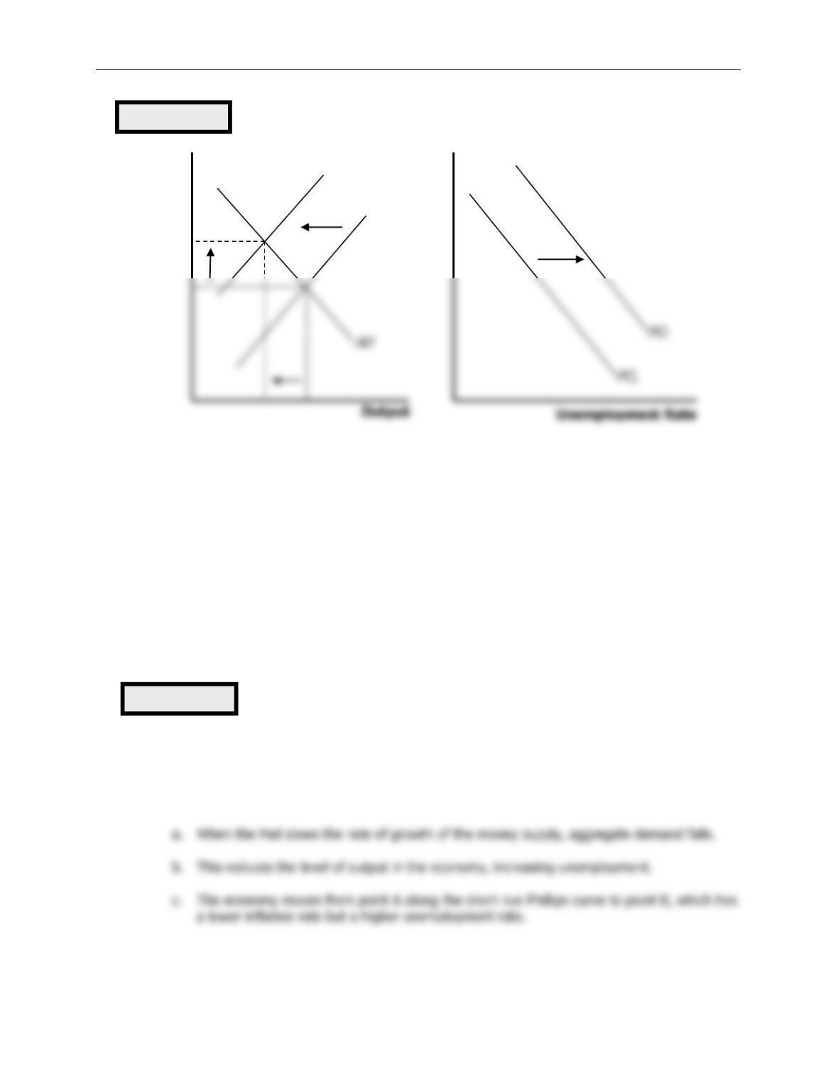
• When the Fed contracts growth in the money supply to reduce inflation, it moves the economy along
the short-run Phillips curve, which results in temporarily high unemployment. The cost of disinflation
depends on how quickly expectations of inflation fall. Some economists argue that a credible
commitment to low inflation can reduce the cost of disinflation by inducing a quick adjustment of
expectations.
CHAPTER OUTLINE:
I. The Phillips Curve
A. Origins of the Phillips Curve
1. In 1958, economist A. W. Phillips published an article discussing the negative correlation
between inflation rates and unemployment rates in the United Kingdom.
2. American economists Paul Samuelson and Robert Solow showed a similar relationship
between inflation and unemployment for the United States two years later.
3. The belief was that low unemployment is related to high aggregate demand, and high
Chapter 22/The Short-Run Trade-off between Inflation and Unemployment ❖ 391
B. Aggregate Demand, Aggregate Supply, and the Phillips Curve
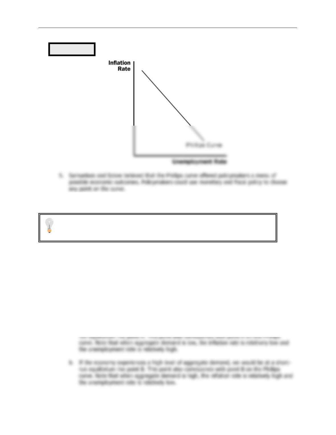
1. The Phillips curve shows the combinations of inflation and unemployment that arise in the
short run as shifts in the aggregate-demand curve move the economy along the short-run
aggregate-supply curve.
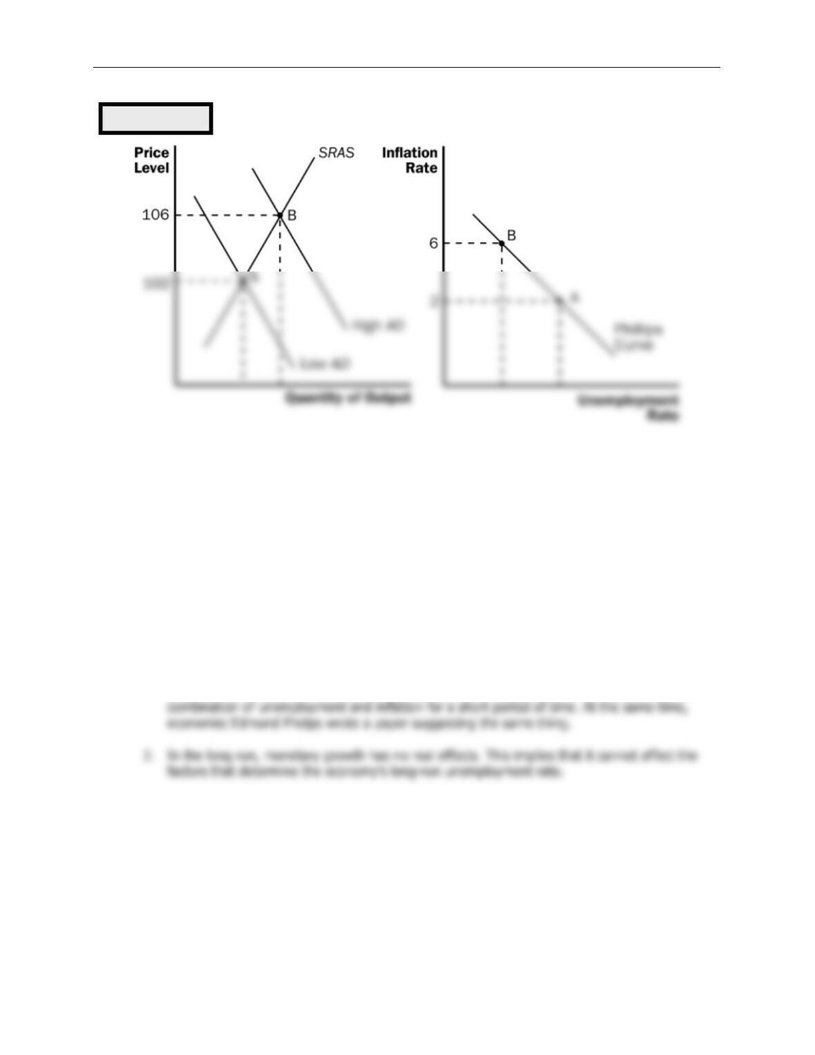
2. The greater the aggregate demand for goods and services, the greater the economy’s output
and the higher the price level. Greater output means lower unemployment. The higher the
price level in the current year, the higher the rate of inflation.
3. Example: The price level is 100 (measured by the Consumer Price Index) in the year 2020.
There are two possible changes in the economy for the year 2021: a low level of aggregate
demand or a high level of aggregate demand.
a. If the economy experiences a low level of aggregate demand, we would be at a short–
Figure 1
Show how the Phillips curve is derived from the aggregate demand/aggregate supply
model step by step. This graph is different from all the other graphs that they have
drawn in macroeconomics, because it is not a supply-and-demand diagram.
392 ❖ Chapter 22/The Short-Run Trade-off between Inflation and Unemployment
4. Because monetary and fiscal policies both shift the aggregate-demand curve, these policies
can move the economy along the Phillips curve.
a. Increases in the money supply, increases in government spending, or decreases in taxes
all increase aggregate demand and move the economy to a point on the Phillips curve
with lower unemployment and higher inflation.
b. Decreases in the money supply, decreases in government spending, or increases in taxes
all lower aggregate demand and move the economy to a point on the Phillips curve with
higher unemployment and lower inflation.
II. Shifts in the Phillips Curve: The Role of Expectations
A. The Long-Run Phillips Curve
1. In 1968, economist Milton Friedman argued that monetary policy is only able to choose a
Figure 2
Chapter 22/The Short-Run Trade-off between Inflation and Unemployment ❖ 393
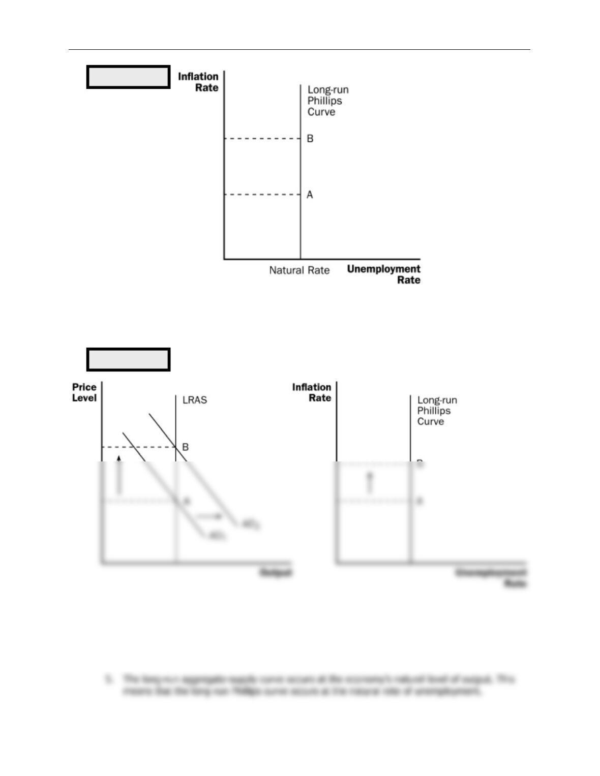
3. Thus, in the long run, we would not expect there to be a relationship between
unemployment and inflation. This must mean that, in the long run, the Phillips curve is
vertical.
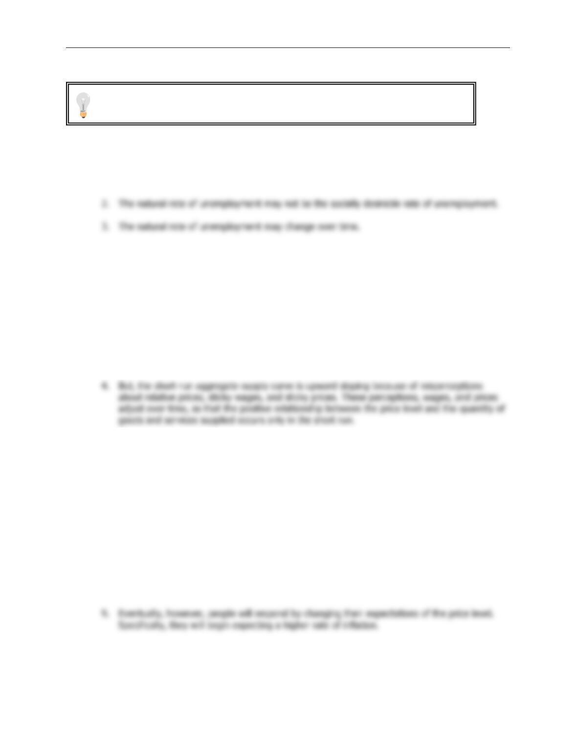
4. The vertical Phillips curve occurs because, in the long run, the aggregate supply curve is
vertical as well. Thus, increases in aggregate demand lead only to changes in the price level
and have no effect on the economy’s level of output. Thus, in the long run, unemployment
will not change when aggregate demand changes, but inflation will.
Figure 3
Figure 4
394 ❖ Chapter 22/The Short-Run Trade-off between Inflation and Unemployment
B. The Meaning of “Natural”
1. Friedman and Phelps considered the natural rate of unemployment to be the rate toward
which the economy gravitates in the long run.
C. Reconciling Theory and Evidence
1. The conclusion of Friedman and Phelps that there is no long-run trade-off between inflation
and unemployment was based on
theory
, while the correlation between inflation and
unemployment found by Phillips, Samuelson, and Solow was based on actual
evidence
.
2. Friedman and Phelps believed that an inverse relationship between inflation and
unemployment exists in the short run.
3. The long-run aggregate-supply curve is vertical, indicating that the price level does not
influence output in the long run.
5. This same logic applies to the Phillips curve. The trade-off between inflation and
unemployment holds only in the short run.
6. The expected level of inflation is an important factor in understanding the difference between
the long-run and the short-run Phillips curves. Expected inflation measures how much people
expect the overall price level to change.
7. The expected rate of inflation is one variable that determines the position of the short-run
aggregate-supply curve. This is true because the expected price level affects the perceptions
of relative prices that people form and the wages and prices that they set.
8. In the short run, expectations are somewhat fixed. Thus, when the Fed increases the money
supply, aggregate demand increases along the upward sloping short-run aggregate-supply
curve. Output grows (unemployment falls) and the price level rises (inflation increases).
You may want to review what is meant by the “natural rate” of unemployment.
Chapter 22/The Short-Run Trade-off between Inflation and Unemployment ❖ 395
D. The Short-Run Phillips Curve
1. We can relate the actual unemployment rate to the natural rate of unemployment, the actual
inflation rate, and the expected inflation rate using the following equation:
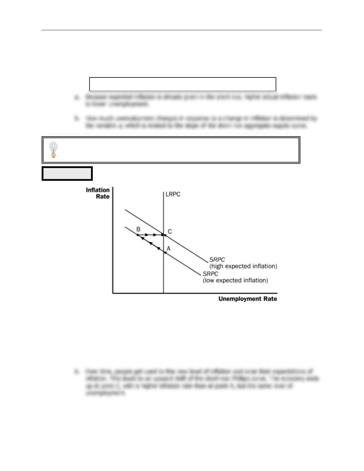
2. If policymakers want to take advantage of the short-run trade-off between unemployment
and inflation, it may lead to negative consequences.
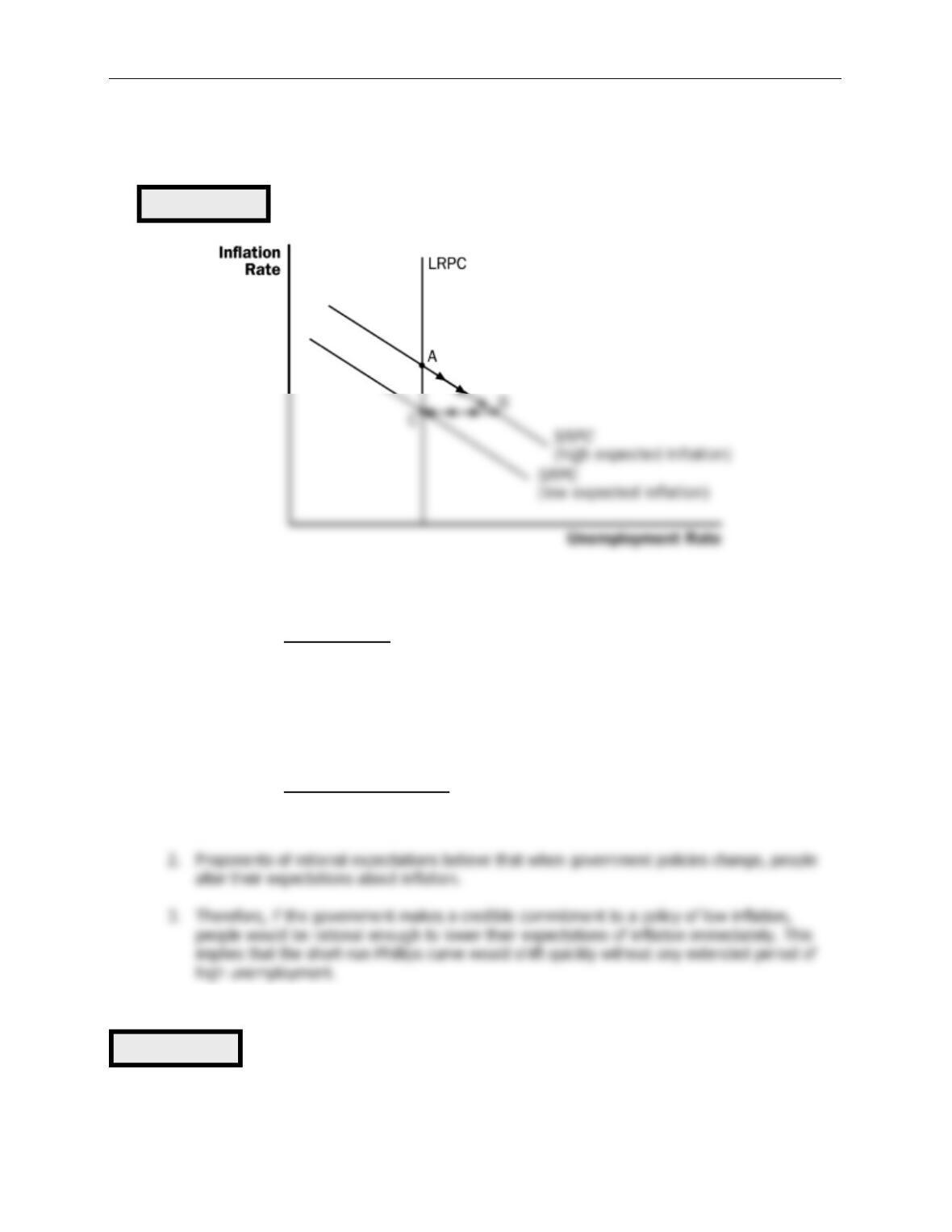
a. Suppose the economy is at point A and policymakers wish to lower the unemployment
rate. Expansionary monetary policy or fiscal policy is used to shift aggregate demand to
the right. The economy moves to point B, with a lower unemployment rate and a higher
rate of inflation.
unemp. rate natural rate (actual inflation expected inflation)
a
= − −
Figure 5
Be sure to discuss why actual inflation always equals expected inflation along the
long-run Phillips curve.
396 ❖ Chapter 22/The Short-Run Trade-off between Inflation and Unemployment
E. The Natural Experiment for the Natural-Rate Hypothesis
1. Definition of the natural-rate hypothesis: the claim that unemployment eventually
returns to its normal, or natural rate, regardless of the rate of inflation.
2. Figure 6 shows the unemployment and inflation rates from 1961 to 1968. It is easy to see
the inverse relationship between these two variables.
3. Beginning in the late 1960s, the government followed policies that increased aggregate
demand.
a. Figure 7 shows the unemployment and inflation rates from 1961 to 1973. The simple
inverse relationship between these two variables began to disappear around 1970.
b. Inflation expectations adjusted to the higher rate of inflation and the unemployment rate
returned to its natural rate of around 5% to 6%.
III. Shifts in the Phillips Curve: The Role of Supply Shocks
A. In 1974, OPEC increased the price of oil sharply. This increased the cost of producing many
goods and services and therefore resulted in higher prices.
Figure 6
Figure 7
Chapter 22/The Short-Run Trade-off between Inflation and Unemployment ❖ 397
B. Given this turn of events, policymakers are left with a less favorable short-run trade-off between
unemployment and inflation.
1. If they increase aggregate demand to fight unemployment, they will raise inflation further.
2. If they lower aggregate demand to fight inflation, they will raise unemployment further.
C. This less favorable trade-off between unemployment and inflation can be shown by a shift of the
short-run Phillips curve. The shift may be permanent or temporary, depending on how people
adjust their expectations of inflation.
D. During the 1970s, the Fed decided to accommodate the supply shock by increasing the supply of
money. This increased the level of expected inflation. Figure 9 shows inflation and unemployment
in the United States during the late 1970s and early 1980s.
IV. The Cost of Reducing Inflation
A. The Sacrifice Ratio
1. To reduce the inflation rate, the Fed must follow contractionary monetary policy.
Figure 8
Figure 9
Price
Level
Inflation
Rate
AS
1
AS
2
1
398 ❖ Chapter 22/The Short-Run Trade-off between Inflation and Unemployment
d. Over time, people begin to adjust their inflation expectations downward and the short–
run Phillips curve shifts. The economy moves from point B to point C, where inflation is
lower and the unemployment rate is back to its natural rate.
2. Therefore, to reduce inflation, the economy must suffer through a period of high
unemployment and low output.
3. Definition of sacrifice ratio: the number of percentage points of annual output lost
in the process of reducing inflation by one percentage point.
4. A typical estimate of the sacrifice ratio is five. This implies that for each percentage point
inflation is decreased, output falls by 5%.
B. Rational Expectations and the Possibility of Costless Disinflation
1. Definition of rational expectations: the theory according to which people optimally
use all the information they have, including information about government
policies, when forecasting the future.
C. The Volcker Disinflation
1. Figure 11 shows the inflation and unemployment rates that occurred while Paul Volcker
worked at reducing the level of inflation during the 1980s.
Figure 10
Figure 11
Chapter 22/The Short-Run Trade-off between Inflation and Unemployment ❖ 399
2. As inflation fell, unemployment rose. In fact, the United States experienced its deepest
recession since the Great Depression.
3. Some economists have offered this as proof that the idea of a costless disinflation suggested
by rational-expectations theorists is not possible. However, there are two reasons why we
might not want to reject the rational-expectations theory so quickly.
a. The cost (in terms of lost output) of the Volcker disinflation was not as large as many
economists had predicted.
D. The Greenspan Era
1. Figure 12 shows the inflation and unemployment rate from 1984 to 2005, called the
Greenspan era because Alan Greenspan became the chairman of the Federal Reserve in
1987.
2. In 1986, OPEC’s agreement with its members broke down and oil prices fell. The result of
this favorable supply shock was a drop in both inflation and unemployment.
3. The rest of the 1990s witnessed a period of economic prosperity. Inflation gradually dropped,
approaching zero by the end of the decade. Unemployment also reached a low level, leading
many people to believe that the natural rate of unemployment had fallen.
E. A Financial Crisis Takes Us for a Ride Along the Phillips Curve
1. In his first couple of years as Fed chairman, Bernanke faced some significant economic
challenges.
a. One challenge arose from problems in the housing and financial markets.
b. The resulting financial crisis led to a large drop in aggregate demand and high rates of
unemployment.
c. Figure 13 shows the implications of these events for inflation and unemployment.
Figure 12