363
WHAT’S NEW IN THE SIXTH EDITION:
A new
In the News
box on “Backward–sloping Labor Supply in Kiribati” has been added.
LEARNING OBJECTIVES:
By the end of this chapter, students should understand:
➢ how a budget constraint represents the choices a consumer can afford.
➢ how indifference curves can be used to represent a consumer’s preferences.
CONTEXT AND PURPOSE:
Chapter 21 is the first of two unrelated chapters that introduce students to advanced topics in
microeconomics. These two chapters are intended to whet their appetites for further study in economics.
Chapter 21 is devoted to an advanced topic known as the theory of consumer choice.
THE THEORY OF CONSUMER
CHOICE
21
364 ❖ Chapter 21/The Theory of Consumer Choice
KEY POINTS:
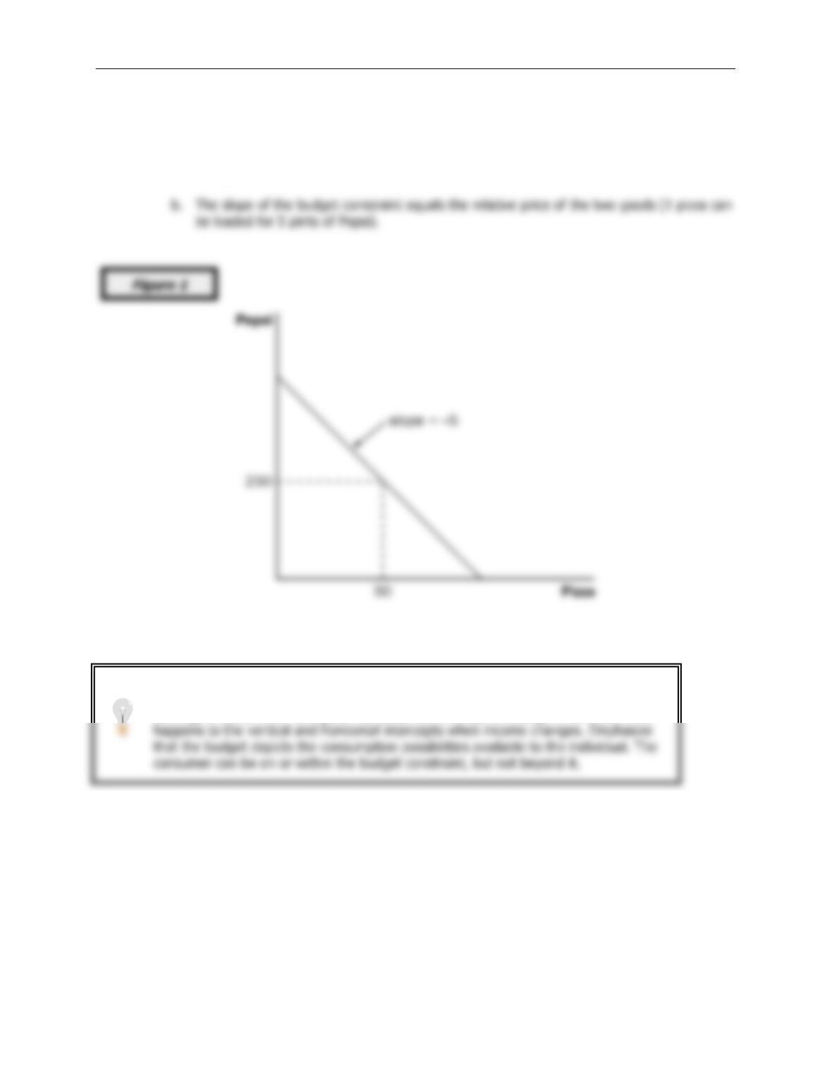
• A consumer’s budget constraint shows the possible combinations of different goods he can buy given
his income and the prices of the goods. The slope of the budget constraint equals the relative price
of the goods.
• The consumer optimizes by choosing the point on his budget constraint that lies on the highest
indifference curve. At this point, the slope of the indifference curve (the marginal rate of substitution
between the goods) equals the slope of the budget constraint (the relative price of the goods).
• The theory of consumer choice can be applied in many situations. It explains why demand curves can
potentially slope upward, why higher wages could either increase or decrease the quantity of labor
supplied, and why higher interest rates could either increase or decrease saving.
CHAPTER OUTLINE:
I. The Budget Constraint: What the Consumer Can Afford
A. Example: A consumer has an income of $1,000 per month to spend on pizza and Pepsi. The price
of a pizza is $10 and the price of a pint of Pepsi is $2.
This chapter is an advanced treatment of consumer choice using indifference curve
The best way to develop this model is to use specific examples with definite
quantities, prices, and levels of income.
Chapter 21/The Theory of Consumer Choice ❖ 365
D. Using this information, we can draw the consumer’s budget constraint.
a. The slope of the budget constraint measures the rate at which the consumer can trade
one good for another.
Although the book does it later, now might be a good time to show the effects of
price and income changes. Show mathematically and graphically how a doubling (or
halving) of the price of one good will cause its intercept to change. Also show what

366 ❖ Chapter 21/The Theory of Consumer Choice
II. Preferences: What the Consumer Wants
Activity 1—You Can’t Always Get What You Want
Type: In-class activity
Topics: Budget constraints
Materials needed: None
Time: 5 minutes
Class limitations: Works in any size class
Purpose
This activity shows consumers are restricted by their limited incomes and by the prices of
goods.
Instructions
Ask the students to think about maximizing their own utility.
The answer, of course, is they cannot afford it. Consumers’ purchases are constrained by
their incomes.
However, that is not the only constraint. Ask them to estimate the cost of their selected items
and write it next to the items. Now, have them assume Bill Gates is too busy to go shopping,
so he gives them the money instead. He does not put any restrictions on the use of the cash;
all he wants is to see them maximize their happiness.
Points for Discussion
1) Consumers have limited income.
2) Goods have prices.
Together these things determine the consumer’s budget constraint.
Chapter 21/The Theory of Consumer Choice ❖ 367
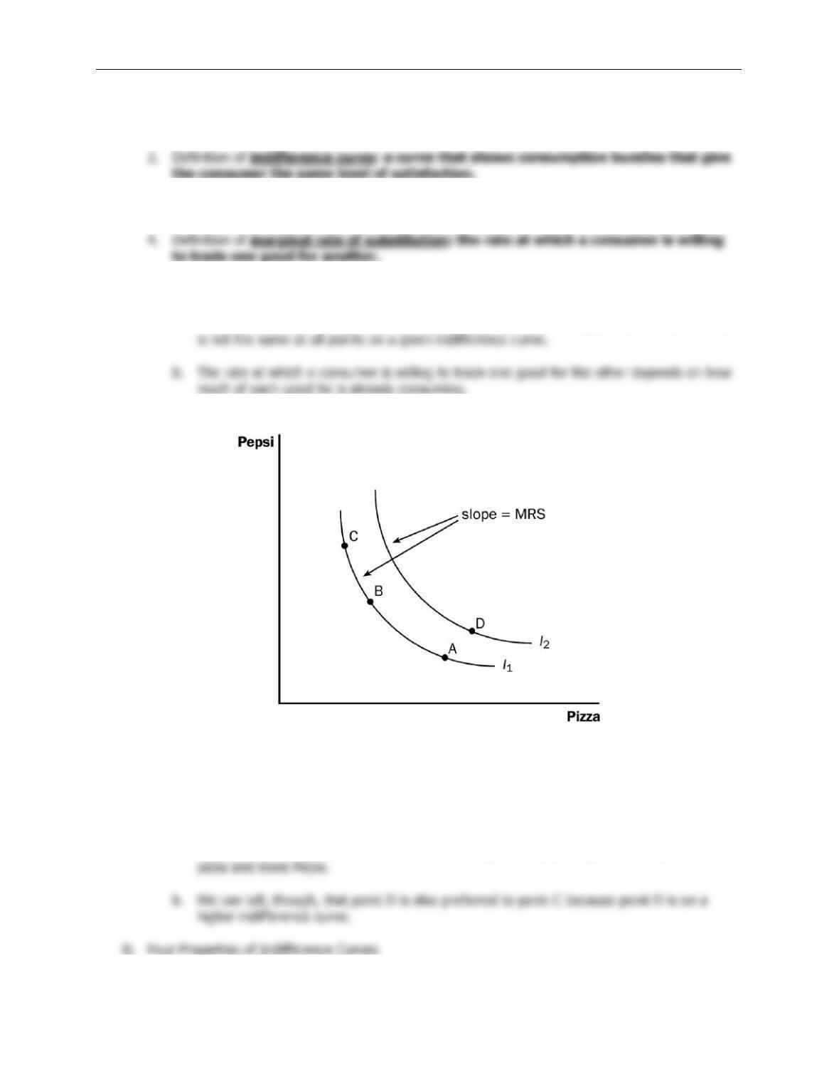
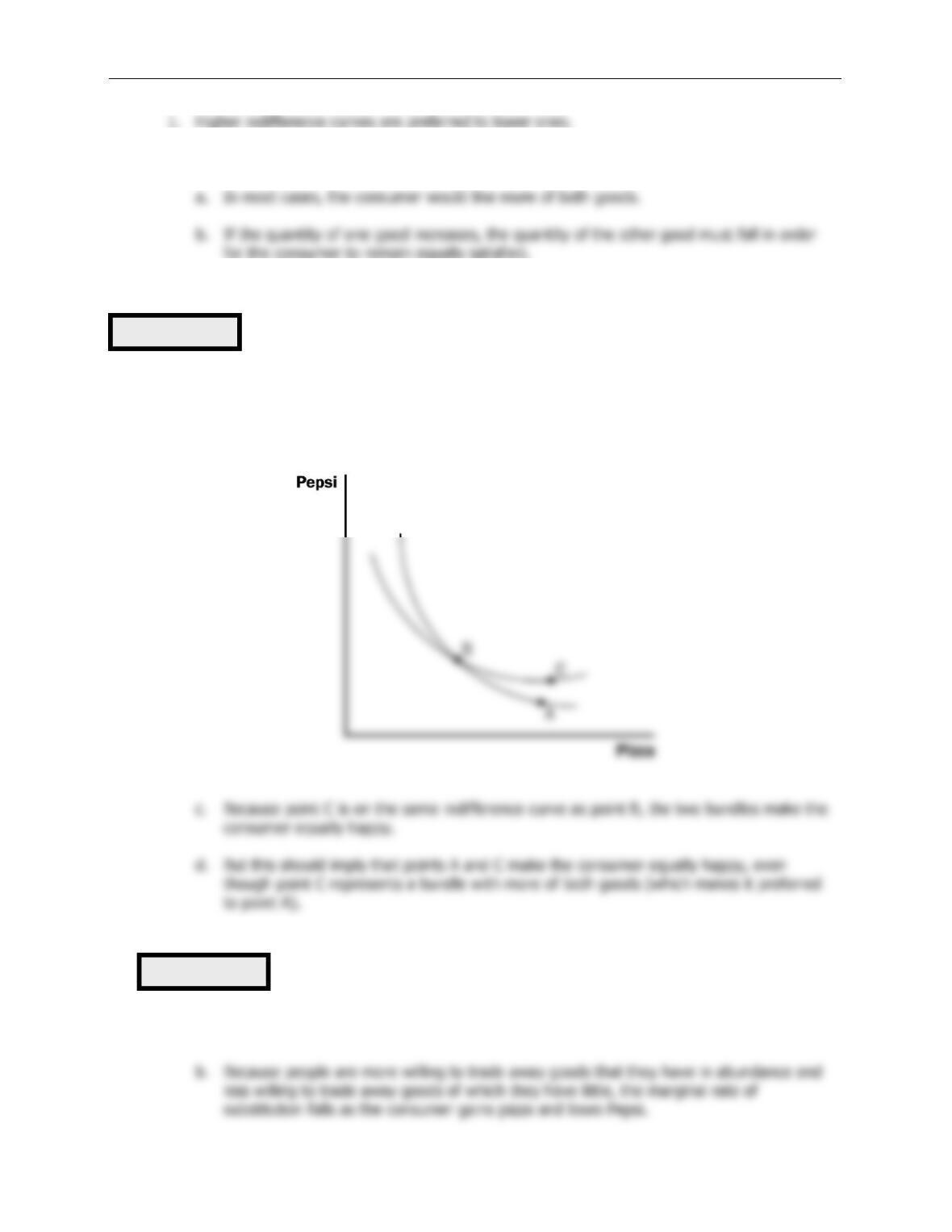
1. A consumer is indifferent between two bundles of goods and services if the two bundles suit
his tastes equally well.
3. The consumer is indifferent among points A, B, and C.
5. The marginal rate of substitution is equal to the slope of the indifference curve at any point.
a. Because these indifference curves are not straight lines, the marginal rate of substitution
6. A consumer’s set of indifference curves gives a complete ranking of the consumer’s
preferences.
7. Any point on indifference curve
I
2 will be preferred to any point on indifference curve
I
1.
a. It is obvious that point D would be preferred to point A because point D contains more
368 ❖ Chapter 21/The Theory of Consumer Choice
2. Indifference curves are downward sloping.
3. Indifference curves do not cross.
a. The easiest way to prove this is by showing what would happen if they did cross.
b. Because point A is on the same indifference curve as point B, the two bundles make the
consumer equally happy.
4. Indifference curves are bowed inward.
a. The slope of the indifference curve is the rate at which the consumer is willing to trade
one good for another.
Figure 3
Figure 4
Chapter 21/The Theory of Consumer Choice ❖ 369
C. Two Extreme Examples of Indifference Curves
1. Perfect Substitutes
a. Examples: bundles of nickels and dimes.
b. Most likely, a consumer would always be willing to trade one dime for two nickels,
2. Perfect Complements
a. Example: right shoes and left shoes.
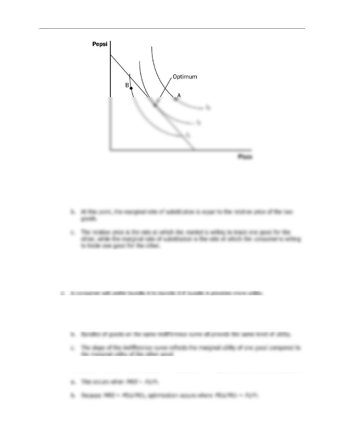
III. Optimization: What the Consumer Chooses
A. The Consumer’s Optimal Choices
1. The consumer would like to end up on the highest possible indifference curve, but he must
also stay within his budget.
3. The optimum point represents the best combination of Pepsi and pizza available to the
consumer.
Figure 5
Figure 6
370 ❖ Chapter 21/The Theory of Consumer Choice
4. At the optimum, the slope of the budget constraint is equal to the slope of the indifference
curve.
a. The indifference curve is tangent to the budget constraint at this point.
B.
FYI: Utility: An Alternative Way to Describe Preferences and Optimization
1. Utility is an abstract measure of the satisfaction that a consumer receives from a bundle of
goods and services.
3. Indifference curves and utility are related.
a. Bundles of goods in higher indifference curves provide a higher level of utility.
4. A consumer can maximize his utility if he ends up on the highest indifference curve possible.
Chapter 21/The Theory of Consumer Choice ❖ 371
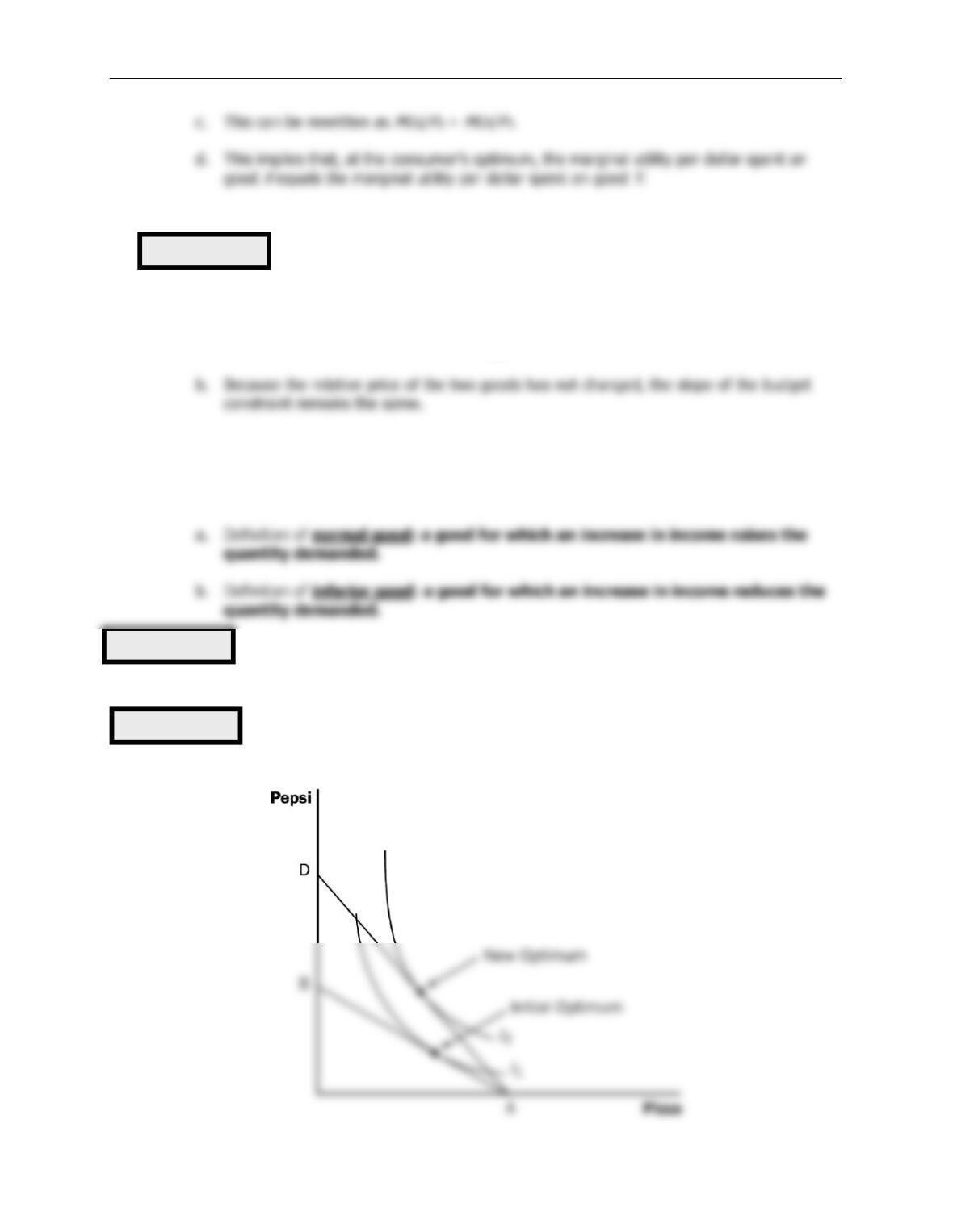
C. How Changes in Income Affect the Consumer’s Choices
1. A change in income shifts the budget constraint.
a. An increase in income can be shown by an outward shift of the budget constraint; a
decrease in income means that the budget constraint shifts inward.
2. An increase in income means that the consumer can now reach a higher indifference curve.
3. Because the consumer increased his consumption of both goods when his income increased,
both Pepsi and pizza must be normal goods.
D. How Changes in Prices Affect the Consumer’s Choices
1. If the price of only one good changes, the budget constraint will tilt.
Figure 7
Figure 8
Figure 9
372 ❖ Chapter 21/The Theory of Consumer Choice
2. Suppose that the price of Pepsi falls from $2 per pint to $1.
a. If the consumer spends his entire income on pizza, the change in the price of Pepsi will
not affect his ability to buy pizza, so point A on the budget constraint remains the same.
3. How such a change in the price of one good alters the consumption of both goods depends
on the consumer’s preferences.
E. Income and Substitution Effects
1. Definition of income effect: the change in consumption that results when a price
change moves the consumer to a higher or lower indifference curve.
a. The decrease in the price of Pepsi will make the consumer better off. Thus, if pizza and
Pepsi are both normal goods, the consumer will want to spread this improvement in his
purchasing power over both goods. This is the income effect and will make the consumer
want to buy more of both goods.
Figure 10
Table 1
Chapter 21/The Theory of Consumer Choice ❖ 373
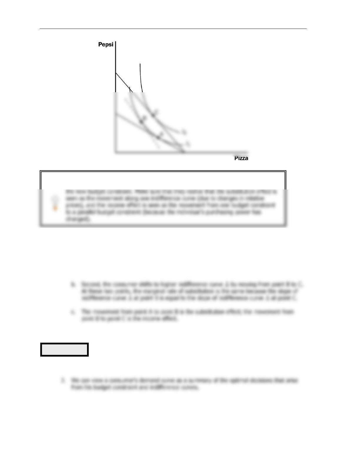
4. We can graphically decompose the change in the consumer’s decision into the income effect
and the substitution effect.
a. First, the consumer moves from the initial optimum (point A) to point B. The consumer is
equally happy at either of these points, but the marginal rate of substitution at point B
reflects the new relative prices of the two goods.
F. Deriving the Demand Curve
1. A demand curve shows how the price of a good affects the quantity demanded.
Figure 11
Students can learn to separate the substitution effects easily if they follow a simple
rule: Have them draw a line tangent to the original indifference curve but parallel to
374 ❖ Chapter 21/The Theory of Consumer Choice
3. When the price of Pepsi falls from $2 per pint to $1, the consumer’s budget constraint shifts
outward, leading to both an income effect and a substitution effect. The consumer moves
from point A to point B, increasing his consumption of Pepsi from 50 pints to 150.
IV. Three Applications
A. Do All Demand Curves Slope Downward?
1. The law of demand states that when the price of a good rises, people buy less of it.
3. Example: A consumer spends his entire budget on meat and potatoes. The price of potatoes
rises.
a. The budget constraint will shift in.
b. The substitution effects suggest that the consumer choose more meat and fewer
potatoes.
4. Definition of Giffen good: a good for which an increase in the price raises the
quantity demanded.
5.
Case Study: The Search for Giffen Goods
B. How Do Wages Affect Labor Supply?
Figure 13
Figure 12

Chapter 21/The Theory of Consumer Choice ❖ 375
2. We can show Sally’s budget constraint graphically.
a. On the horizontal axis, we have hours of leisure. On the vertical axis, we have
consumption goods.
3. Sally’s optimum will occur where the highest possible indifference curve is tangent to the
budget constraint.
4. If Sally’s wage increases, her budget constraint will shift outward.
a. The budget constraint will become steeper, because Sally can get more consumption for
every hour of leisure that she gives up.
d. If the substitution effect is greater than the income effect, Sally will decrease leisure and
work more hours if her wage rises. This results in an upward-sloping labor supply curve.
5.
Case Study: Income Effects on Labor Supply: Historical Trends, Lottery Winners, and the
Carnegie Conjecture
a. One hundred years ago, workers worked six days a week. As wages (adjusted for
inflation) have risen, the length of the workweek has fallen. This suggests that a
backward-bending labor supply curve is not unrealistic.
Figure 14
376 ❖ Chapter 21/The Theory of Consumer Choice
6.
In the News: Backward-sloping Labor Supply in Kiribati
a. On the island of Kiribati, when the coconut industry pays more to workers, the workers
spend less time picking coconuts.
C. How Do Interest Rates Affect Household Saving?
1. Example: Sam is planning ahead for retirement. There are two time periods. Currently, Sam
2. We can view “consumption while young” and “consumption while old” as the two goods that
Sam must choose between.
4. We can draw Sam’s budget constraint.
a. On the horizontal axis, we have “consumption when young” and on the vertical axis, we
have “consumption while old.”
6. If the interest rate rises to 20 percent, two possible outcomes could occur.
a. The increase in the interest rate raises the price of “consumption when young.” The
substitution effect suggests that Sam would lower the amount of consumption when
Figure 15
Figure 16