│ TECHNOLOGY 545
CHAPTER 1
TECHNOLOGY:
USING TECHNOLOGY IN STATISTICS
1. From a list of numbers ranging from 1 to 86, randomly select eight of them. Answers will vary.
4. The average of the numbers 0 to 40 is 20. From a list of numbers ranging from 0 to 40, randomly
select seven of them. Repeat this three times. Average these three numbers and compare with the
population average of 20. Answers will vary.
5. Answers will vary.
CHAPTER 2
TECHNOLOGY:
MONTHLY MILK PRODUCTION
1. 2270.5x=
2. 653.2s=
546 TECHNOLOGY │
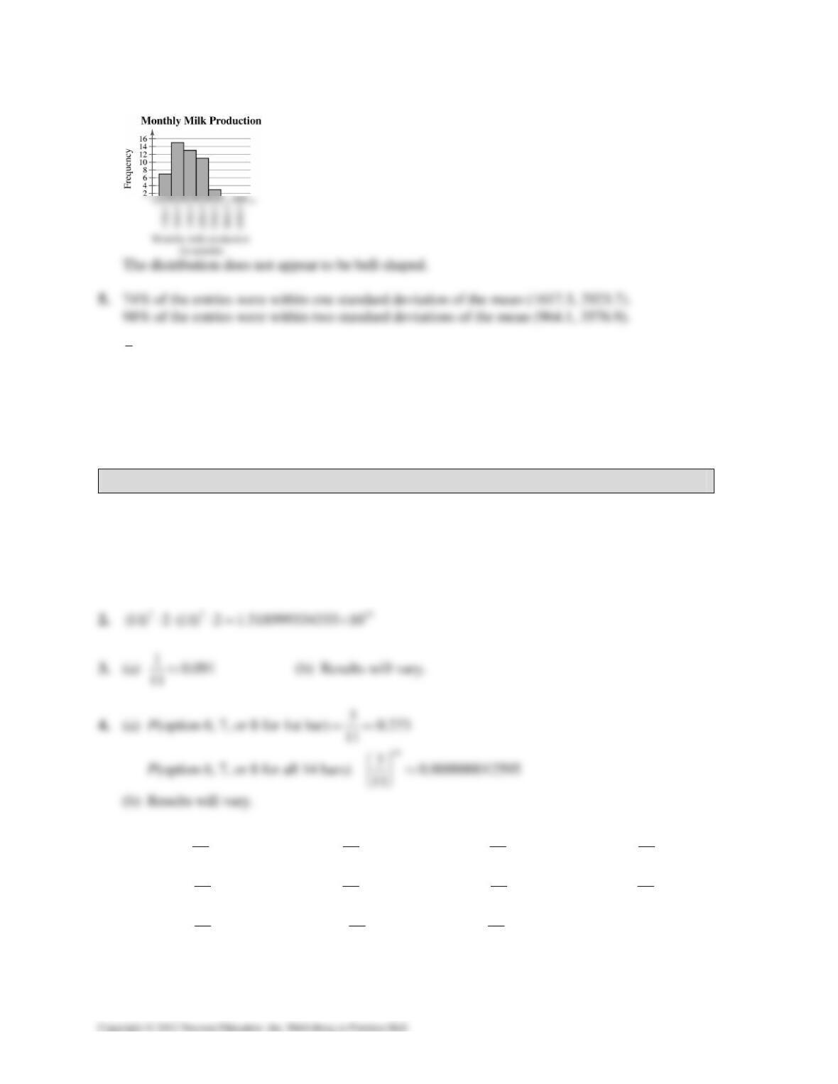
4.
6. 2316.5x=
7. 641.75s≈
8. Answers will vary.
CHAPTER 3
TECHNOLOGY:
SIMULATION: COMPOSING MOZART VARIATIONS WITH
DICE
1. 2 + 11 = 13 phrases were written.
5. (a) 1
(1) 36
P= 2
(2) 36
P= 3
(3) 36
P= 4
(4) 36
P=
5
(5) 36
P= 6
(6) 36
P= 5
(7) 36
P= 4
(8) 36
P=
3
(9) 36
P= 2
(10) 36
P= 1
(1) 36
P=
(b) Results will vary.
│ TECHNOLOGY 547
6. (a) P(option 6, 7, or 8 for 1st bar) 15 0.417
36
=≈
P(option 6, 7, or 8 for all 14 bats)
14
15 0.00000475
36
⎛⎞
⎟
⎜
=≈
⎟
⎜⎟
⎜
⎝⎠
(b) Results will vary.
CHAPTER 4
TECHNOLOGY:
USING POISSON DISTRIBUTIONS AS QUEUING MODELS
1.
x P(x)
0 0.0183
1 0.0733
2 0.1465
10 0.0053
11 0.0019
12 0.0006
13 0.0002
14 0.0001
15 0.0000
2. (a) (See part b) 1, 2, 4, 7
548 TECHNOLOGY │
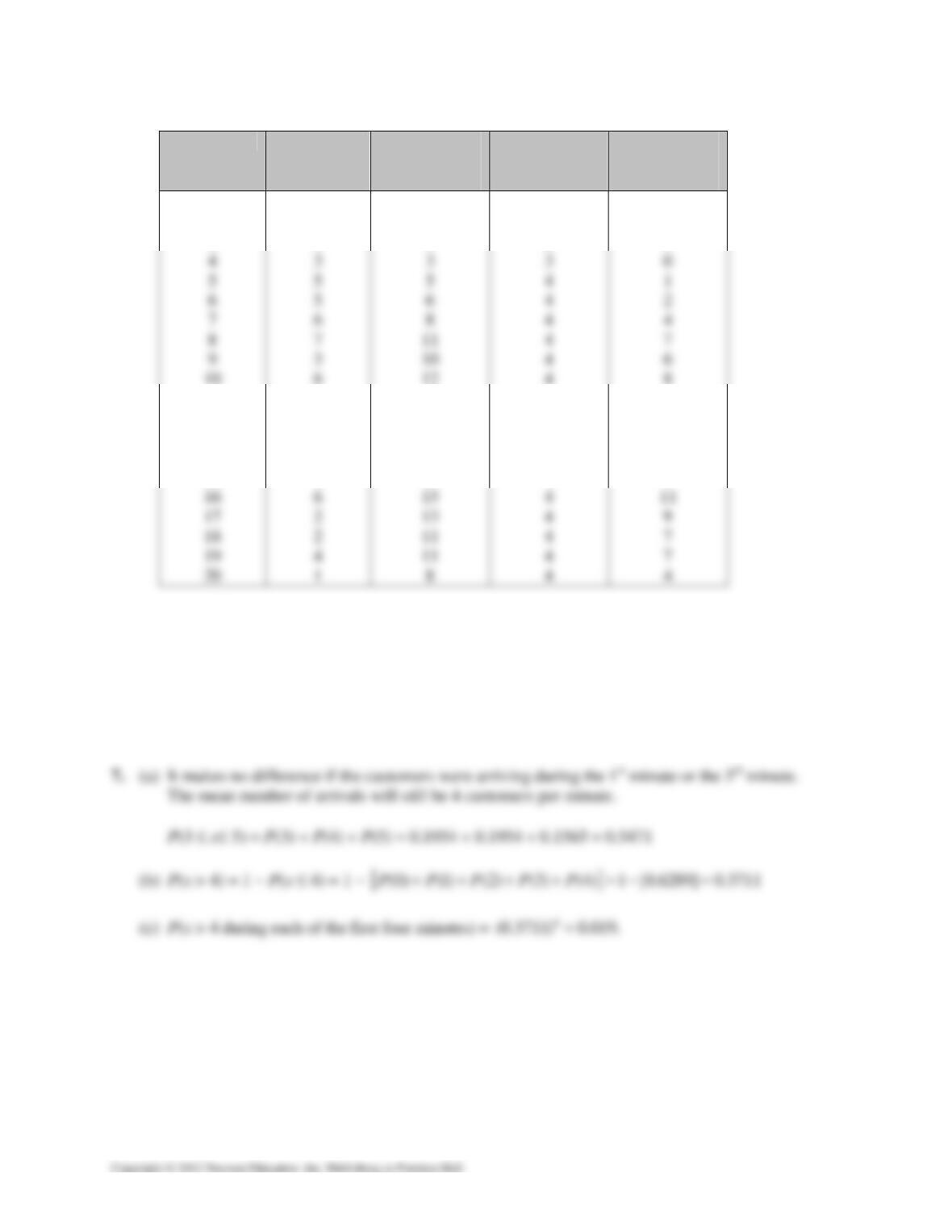
(b)
Minute Customers
at
Checkout
Total
Customers
at Checkout
Customers
Serviced
Customers
Remaining
1
2
3
11
12
13
14
15
3
3
3
3
5
6
3
4
3
3
3
11
12
14
13
13
3
3
3
4
4
4
4
4
4
0
0
0
8
7
8
10
9
9
3. Answers will vary.
4. 20 customers (an additional 1 customer would be forced to wait in line/minute)
5. Answers will vary.
6. P(10) ≈ 0.0181
│ TECHNOLOGY 549
CHAPTER 5
TECHNOLOGY:
AGE DISTRIBUTION IN THE UNITED STATES
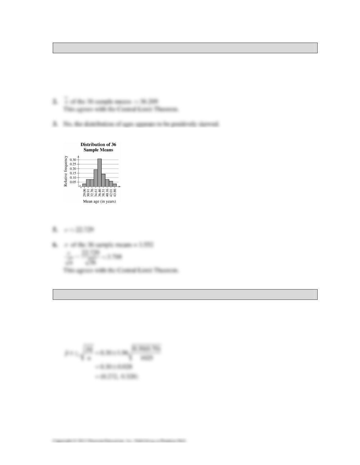
1. 37.06µ≈
4.
The distribution is approximately bell-shaped and symmetrical. This agrees with the Central
Limit Theorem.
CHAPTER 6
TECHNOLOGY:
MOST ADMIRED POLLS
1. ˆ0.30
p=
550 TECHNOLOGY │
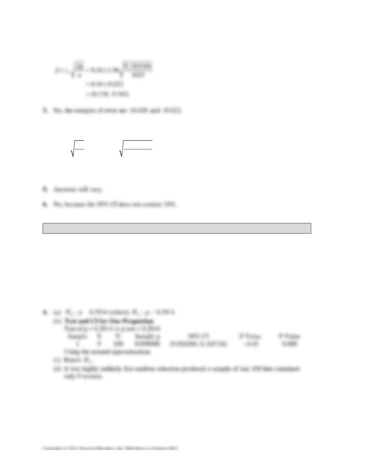
2. ˆ0.16p=
4. ˆ0.15
p=
ˆˆ 0.15(0.85)
ˆ0.15 1.96 1025
0.15 0.022
(0.128, 0.172)
c
pq
pz n
±=±
≈±
=
CHAPTER 7
TECHNOLOGY:
THE CASE OF THE VANISHING WOMEN
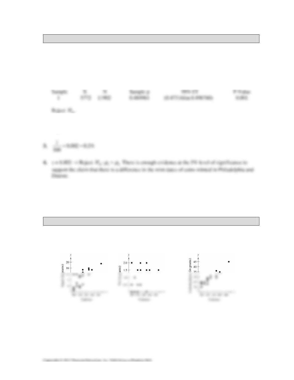
1. Reject 0
H with a P–value less than 0.01.
2. Type I error
3. Sampling process was non-random.
│ TECHNOLOGY 551
CHAPTER 8
TECHNOLOGY:
TAILS OVER HEADS
1. CI for One Proportion
Test of p = 0.5 vs. p not = 0.5
2. Yes, obtaining 5772 heads very uncommon occurrence (see sampling distribution). The coins
might not be fair.
µ
5. z = 1.010 → Fail to reject 01 2
:H
µ
µ
= There is not enough evidence at the 5% level of
significance to support the claim that there is a difference in the value of coins minted in
Philadelphia and Denver.
CHAPTER 9
TECHNOLOGY:
NUTRIENTS IN BREAKFAST CEREALS
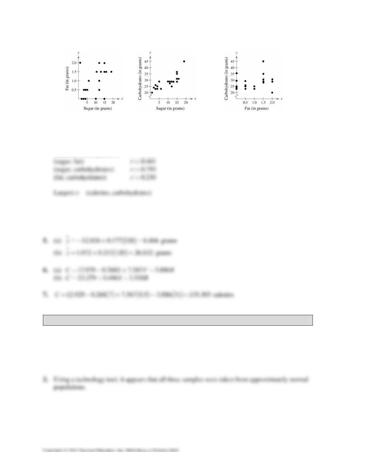
1. (a) (b) (c)
552 TECHNOLOGY │
(d) (e) (f)
2. (calories, sugar), (calories, carbohydrates), (sugar, carbohydrates)
3. (calories, sugar): 0.766r≈
(calories, fat): 0.415r≈
(calories, carbohydrates): 0.913r≈
4. (a)
12.836 0.177yx=− +
(b)
1.072 0.213yx=+
CHAPTER 10
TECHNOLOGY:
TEACHER SALARIES
1. Yes, because the salaries are from different states, it is safe to assume that the samples are
independent.
│ TECHNOLOGY 553
3. 22 22
01 2 1 20
:,:(2.86)
a
HHF
σσ σσ
=≠=
(CA, OH) → F ≈ 0.954 → Fail to reject 0.H
(CA, TX) → F ≈ 2.123 → Fail to reject 0.H
(CA, TX) → F ≈ 2.226 → Fail to reject 0.H
5. The sampleS are independent.
22 22
01 2 1 20
:,:(2.86)
a
HHF
σσ σσ
=≠=
(AK, NV) → F ≈ 1.227 → Fail to reject 0.H
(AK, NY) → F ≈ 0.266 → Fail to reject 0.H
(NV, NY) → F ≈ 0.217 → Fail to reject 0.H
CHAPTER 11
TECHNOLOGY:
U.S. INCOME AND ECONOMIC RESEARCH
1.
554 TECHNOLOGY │
2. 0:H median ≤ 30,000
:
a
H median > 30,000 (claim)
The critical value is 2.
3. 0:H There is no difference in incomes in the Northeast and South. (claim)
:
a
H There is a difference in incomes in the Northeast and South.
The critical values are 01.96.z=±
µ
4. 0:H There is no difference in the incomes for all four regions.
:
a
H There is a difference in the incomes for all four regions. (claim)
2
0
χ
= 7.815
│ TECHNOLOGY 555
Analysis of Variance
Variation
Sum of
squares
Degrees of
freedom
Mean
squares
F
P
Between 69,265,161 3 23,088,387 0.53 0.664
Within 1.917 × 10⁹ 44 43,556,858
6. (Box-and-whisker plot)
0:H There is no difference in incomes in the Northeast and South. (claim)
:
a
H There is a difference in incomes in the Northeast and South.
The critical values are 01.96z=± .
11 2
(1)
15(15151) 232.5
nn n
µ
++ ++
===

556 TECHNOLOGY │
(Kruskal-Wallis test)
H = 4.38
Fail to reject 0.H There is not enough evidence at the 5% level of significance to reject the claim
that the distributions of annual incomes four all four regions are the same.
(ANOVA test)
Analysis of Variance
Variation
Sum of
squares
Degrees of
freedom
Mean
squares
F
P
Between 810,166,455 3 270,055,485 1.26 0.297
Within 1.200 × 10¹⁰ 56 214,332,060