Chapter 2
Chapter 2
Section 2.1
2.1.1Not a linear transformation, since y2=x2+ 2 is not linear in our sense.
2.1.5By Theorem 2.1.2, the three columns of the 2 ×3 matrix Aare T(~e1), T (~e2), and T(~e3), so that
A=7 6 −13
11 9 17 .
2.1.8Reducing the system x1+ 7x2=y1
3x1+ 20x2=y2, we obtain x1=−20y1+ 7y2
x2= 3y1−y2.
2.1.10 We have to attempt to solve the equation y1
y2=1 2
4 9 x1
x2for x1and x2. Reducing the system
x1+ 2x2=y1
4x1+ 9x2=y2we find that x1= 9y1+ 2y2
x2=−4y1+y2or x1
x2=9−2
−4 1 y1
y2.
The inverse matrix is 9−2
−4 1 .
50
Section 2.1
2.1.13 a First suppose that a6= 0. We have to attempt to solve the equation y1
y2=a b
c d x1
x2for x1and x2.
ax1+bx2=y1
cx1+dx2=y2÷a→x1+b
ax2=1
ay1
cx1+dx2=y2−c(I)→
x1+b
ax2=1
ay1
(d−bc
a)x2=−c
ay1+y2→
x1+b
ax2=1
ay1
(ad−bc
a)x2=−c
ay1+y2
b First suppose that ad −bc 6= 0 and a6= 0. Let D=ad −bc for simplicity. We continue our work in part (a):
x1+b
ax2=1
ay1
D
ax2=−c
ay1+y2·a
D→
51
Chapter 2
cx1+dx2=y2
bx2=y1÷c
÷b
b0=1
2.1.14 a By Exercise 13a, 2 3
5kis invertible if (and only if) 2k−15 6= 0, or k6= 7.5.
2.1.15 By Exercise 13a, the matrix a−b
b a is invertible if (and only if) a2+b26= 0, which is the case unless
a=b= 0. If a−b
b a is invertible, then its inverse is 1
a2+b2a b
−b a , by Exercise 13b.
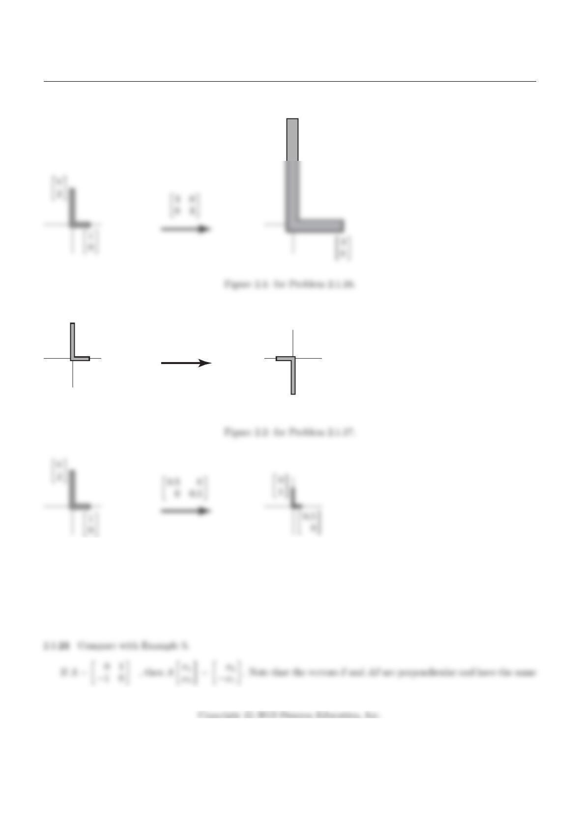
2.1.18 Compare with Exercise 16: This matrix represents a scaling by the factor of 1
2; the inverse is a scaling by 2.
(See Figure 2.3.)
52
Section 2.1
·0
6¸
·0
2¸
·1
0¸
·−1 0
0−1¸·−1
0¸
·0
−2¸
Figure 2.3: for Problem 2.1.18.
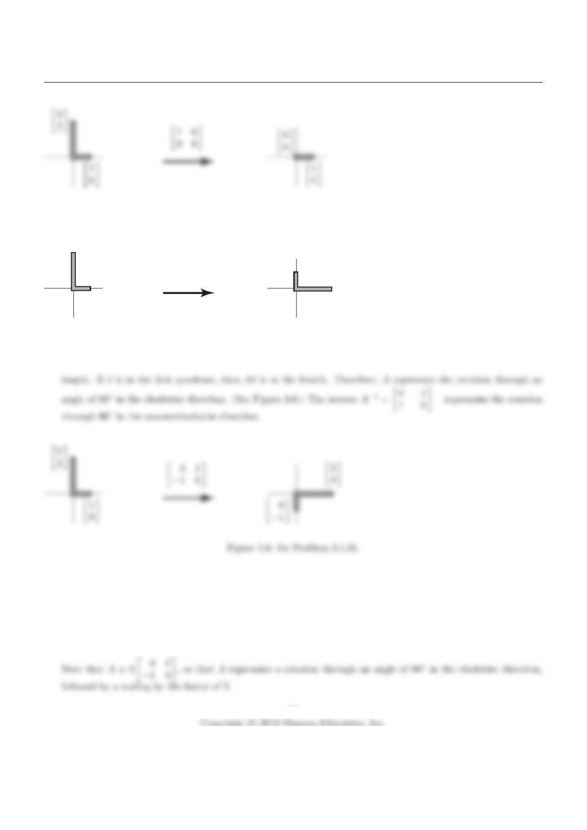
2.1.20 If A=0 1
1 0 , then Ax1
x2=x2
x1, so that Arepresents the reflection about the line x2=x1. This
transformation is its own inverse: A−1=A. (See Figure 2.5.)
53
Chapter 2
Figure 2.4: for Problem 2.1.19.
·0
2¸
·1
0¸
·0 1
1 0 ¸·0
1¸
·2
0¸
Figure 2.5: for Problem 2.1.20.
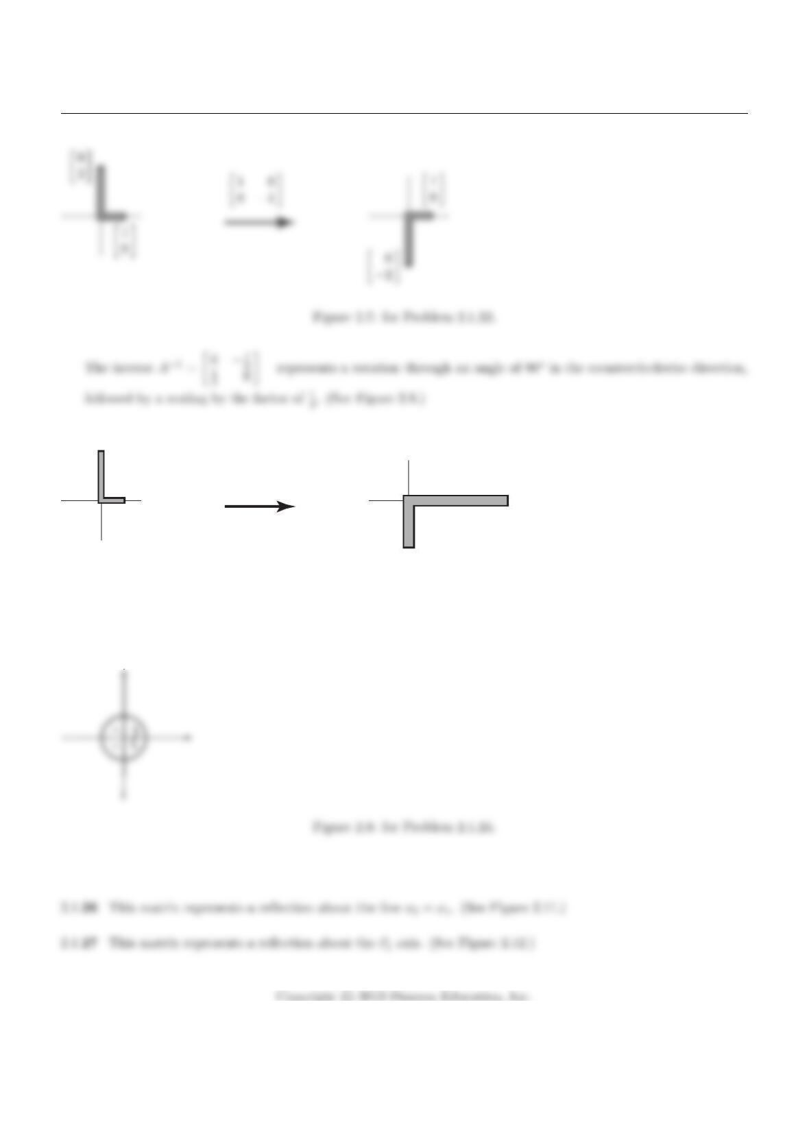
2.1.22 If A=1 0
0−1, then Ax1
x2=x1
−x2, so that Arepresents the reflection about the ~e1axis. This
transformation is its own inverse: A−1=A. (See Figure 2.7.)
2.1.23 Compare with Exercise 21.
54
Section 2.1
·0
2¸
·1
0¸
·0 2
−2 0 ¸
·0
−2¸
·4
0¸
Figure 2.8: for Problem 2.1.23.
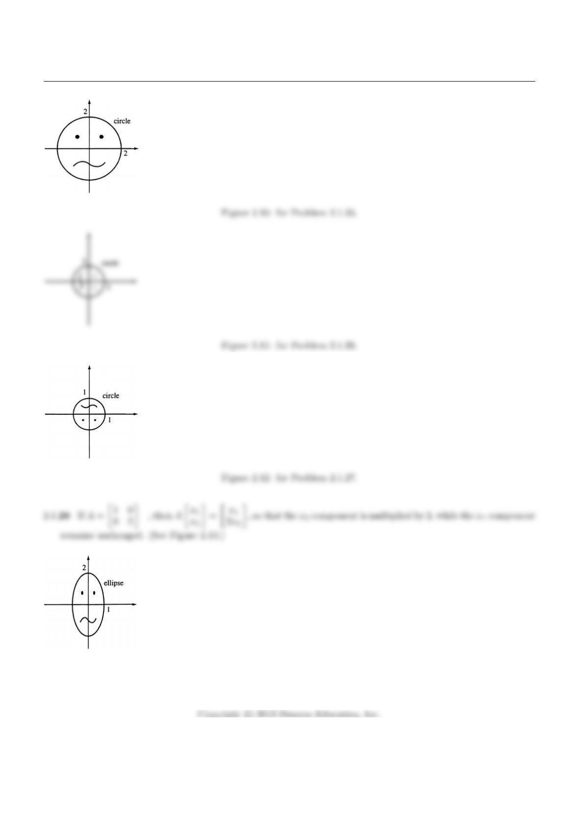
2.1.24 Compare with Example 5. (See Figure 2.9.)
2.1.25 The matrix represents a scaling by the factor of 2. (See Figure 2.10.)
55
Chapter 2
Figure 2.13: for Problem 2.1.28.
56
Section 2.1
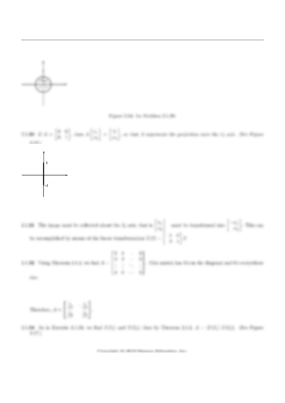
2.1.29 This matrix represents a reflection about the origin. Compare with Exercise 17. (See Figure 2.14.)
2.15.)
Figure 2.15: for Problem 2.1.30.
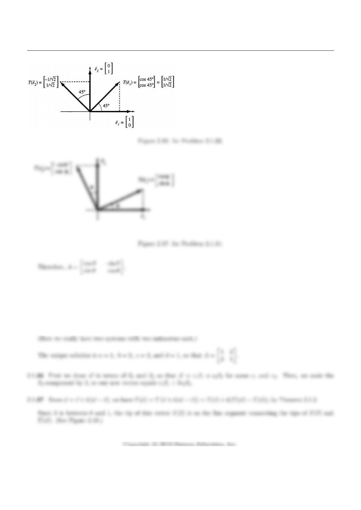
2.1.33 By Theorem 2.1.2, A=T1
0T0
1. (See Figure 2.16.)
57
Chapter 2
2.1.35 We want to find a matrix A=a b
c d such that A5
42 =89
52 and A6
41 =88
53 . This amounts to
solving the system
5a+ 42b= 89
6a+ 41b= 88
5c+ 42d= 52
6c+ 41d= 53
.
58
Section 2.1
2.1.39 By Theorem 2.1.2, we have T
x1
…
xm
=
T(~e1). . . T (~em)
x1
…
xm
=x1T(~e1) + ···+xmT(~em).
2.1.40 These linear transformations are of the form [y] = [a][x], or y=ax. The graph of such a function is a line
through the origin.
59
Chapter 2
2.1.43 aT(~x) =
2
3
4
·
x1
x2
x3
= 2x1+ 3x2+ 4x3= [2 3 4]
x1
x2
x3
The transformation is indeed linear, with matrix [2 3 4].
60
Section 2.1
2.1.45 Yes, ~z =L(T(~x)) is also linear, which we will verify using Theorem 2.1.3. Part a holds, since L(T(~v +~w)) =
L(T(~v) + T(~w)) = L(T(~v)) + L(T(~w)), and part b also works, because L(T(k~v)) = L(kT (~v)) = kL(T(~v)).
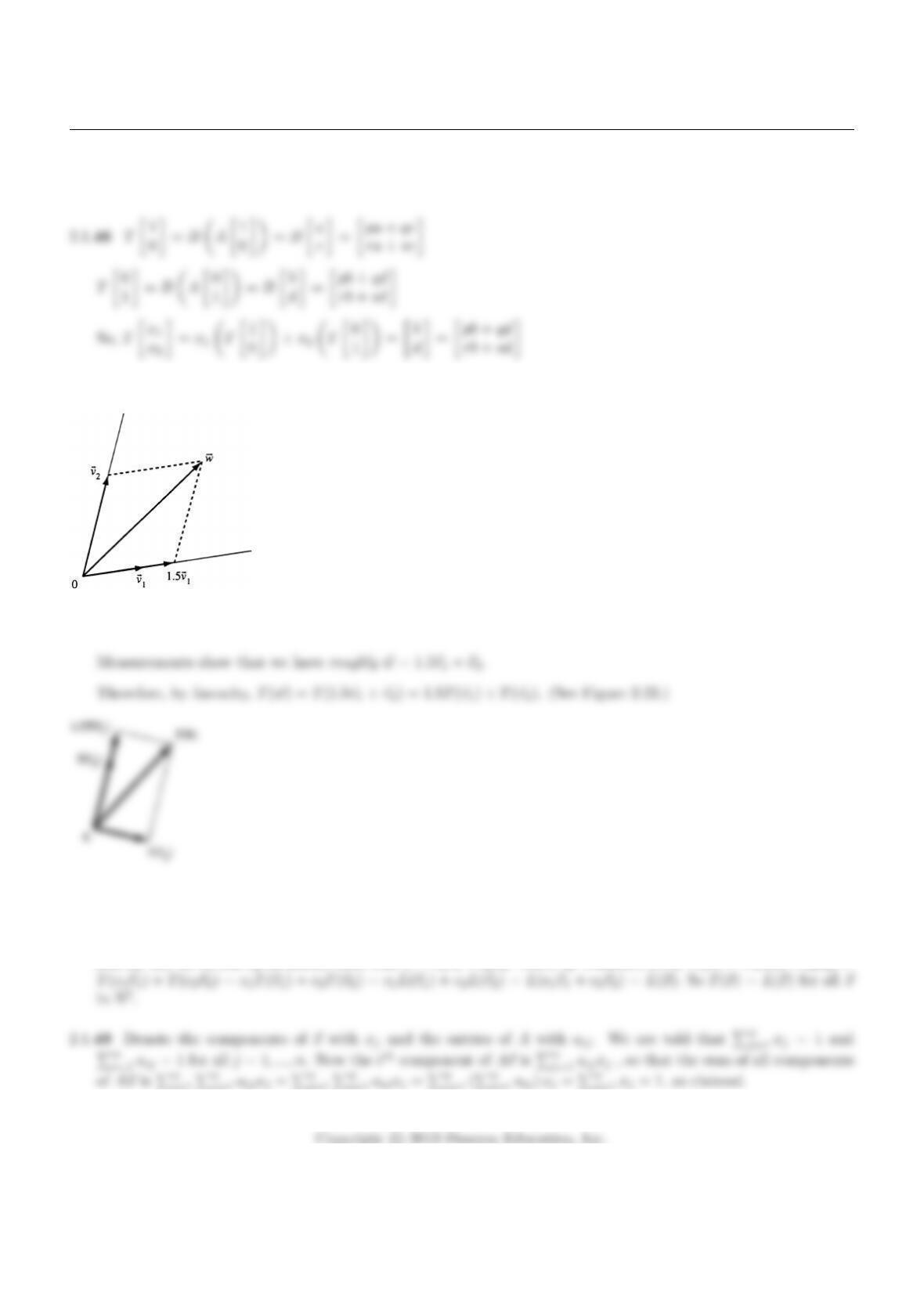
2.1.47 Write ~w as a linear combination of ~v1and ~v2:~w =c1~v1+c2~v2. (See Figure 2.21.)
Figure 2.21: for Problem 2.1.47.
Figure 2.22: for Problem 2.1.47.
2.1.48 Let ~x be some vector in R2.Since ~v1and ~v2are not parallel, we can write ~x in terms of components of ~v1
and ~v2. So, let c1and c2be scalars such that ~x =c1~v1+c2~v2.Then, by Theorem 2.1.3, T(~x) = T(c1~v1+c2~v2) =
i=1 Pn
j=1 aij xj=Pn
j=1 Pn
i=1 aij xj=Pn
j=1 (Pn
i=1 aij )xj=Pn
j=1 xj= 1, as claimed.
61
Chapter 2
Also, the components of A~x are nonnegative since all the scalars aij and xjare nonnegative. Therefore, A~x is a
distribution vector.
2.1.50 Proceeding as in Exercise 51, we find
0100
4
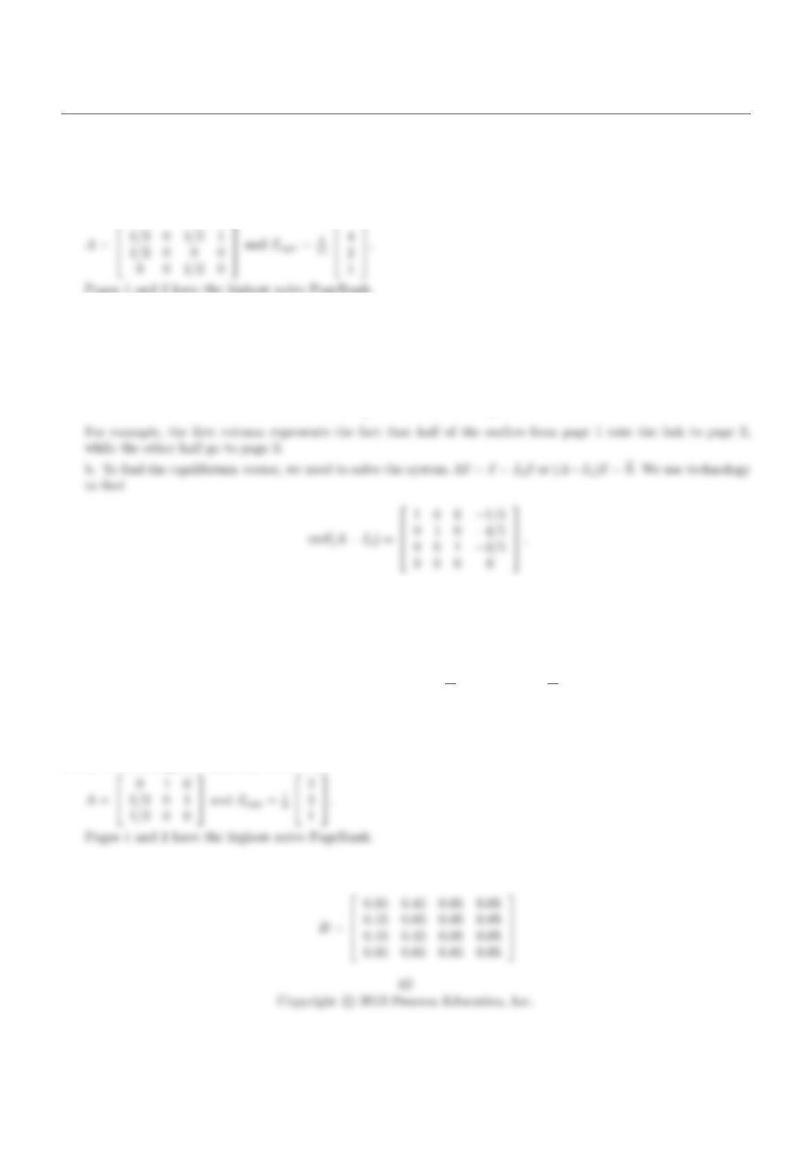
2.1.51 a. We can construct the transition matrix Acolumn by column, as discussed in Example 9:
A=
0 0 1/3 0
1/201/3 1/2
1/2 0 0 1/2
0 1 1/3 0
.
The solutions are of the form ~x =
t
4t
3t
5t
, where tis arbitrary. The distribution vector among these solutions
must satisfy the condition t+ 4t+ 3t+ 5t= 13t= 1, or t=1
13 . Thus ~xequ =1
13
1
4
3
5
.
c. Page 4 has the highest naive PageRank.
2.1.52 Proceeding as in Exercise 51, we find
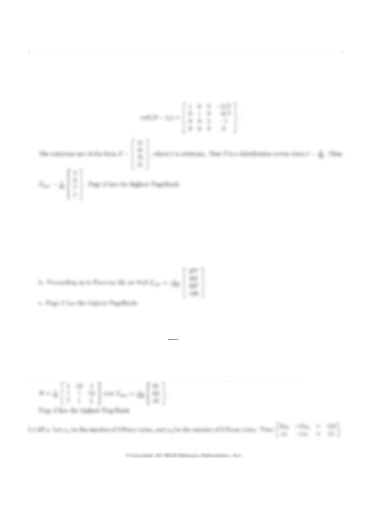
2.1.53 a. Constructing the matrix Bcolumn by column, as explained for the second column, we find
Section 2.1
b. The matrix 0.05Eaccounts for the jumpers, since 5% of the surfers from a given page jump to any other page
(or stay put). The matrix 0.8Aaccounts for the 80% of the surfers who follow links.
c. To find the equilibrium vector, we need to solve the system B~x =~x =I4~x or (B−I4)~x =~
0. We use technology
to find
2.1.54 a. Here we consider the same mini-Web as in Exercise 50. Using the formula for Bfrom Exercise 53b , we
find
B=
0.05 0.85 0.05 0.05
0.45 0.05 0.45 0.85
0.45 0.05 0.05 0.05
0.05 0.05 0.45 0.05
.
2.1.55 Here we consider the same mini-Web as in Exercise 51. Proceeding as in Exercise 53, we find
B=
0.05 0.05 19/60 0.05
0.45 0.05 19/60 0.45
0.45 0.05 0.05 0.45
0.05 0.85 19/60 0.05
and ~xequ =1
2860
323
855
675
1007
.
Page 4 has the highest PageRank.
2.1.56 Here we consider the same mini-Web as in Exercise 52. Proceeding as in Exercise 53, we find
63
Chapter 2
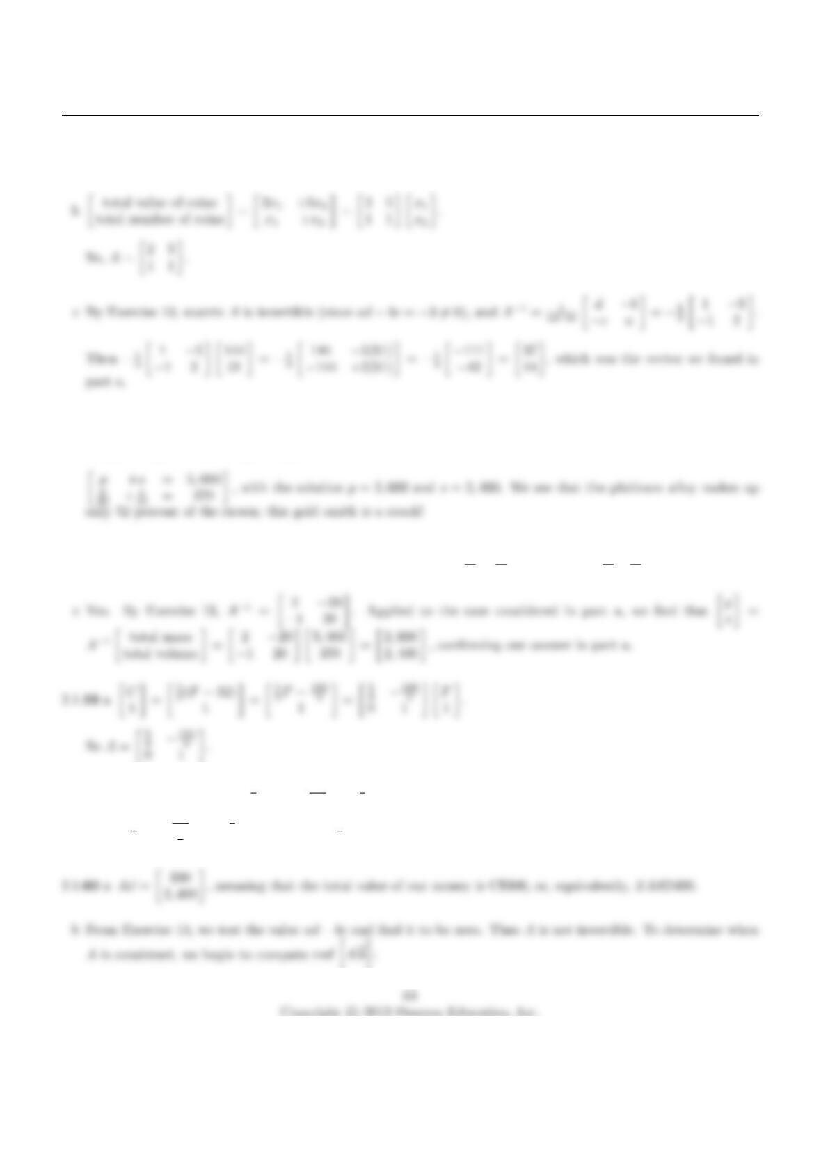
From this we easily find our solution vector to be 37
14 .
2.1.58 a Let p
s=mass of the platinum alloy
mass of the silver alloy . Using the definition density = mass/volume, or volume =
mass/density, we can set up the system:
b We seek the matrix Asuch that Ap
s=total mass
total volume =p+s
p
20 +s
10 . Thus A=1 1
1
20
1
10 .
b Using Exercise 13, we find 5
9(1) −(−160
9)0 = 5
96= 0, so Ais invertible.
A−1=9
51160
9
05
9=9
532
0 1 . So, F=9
5C+ 32.
Section 2.1
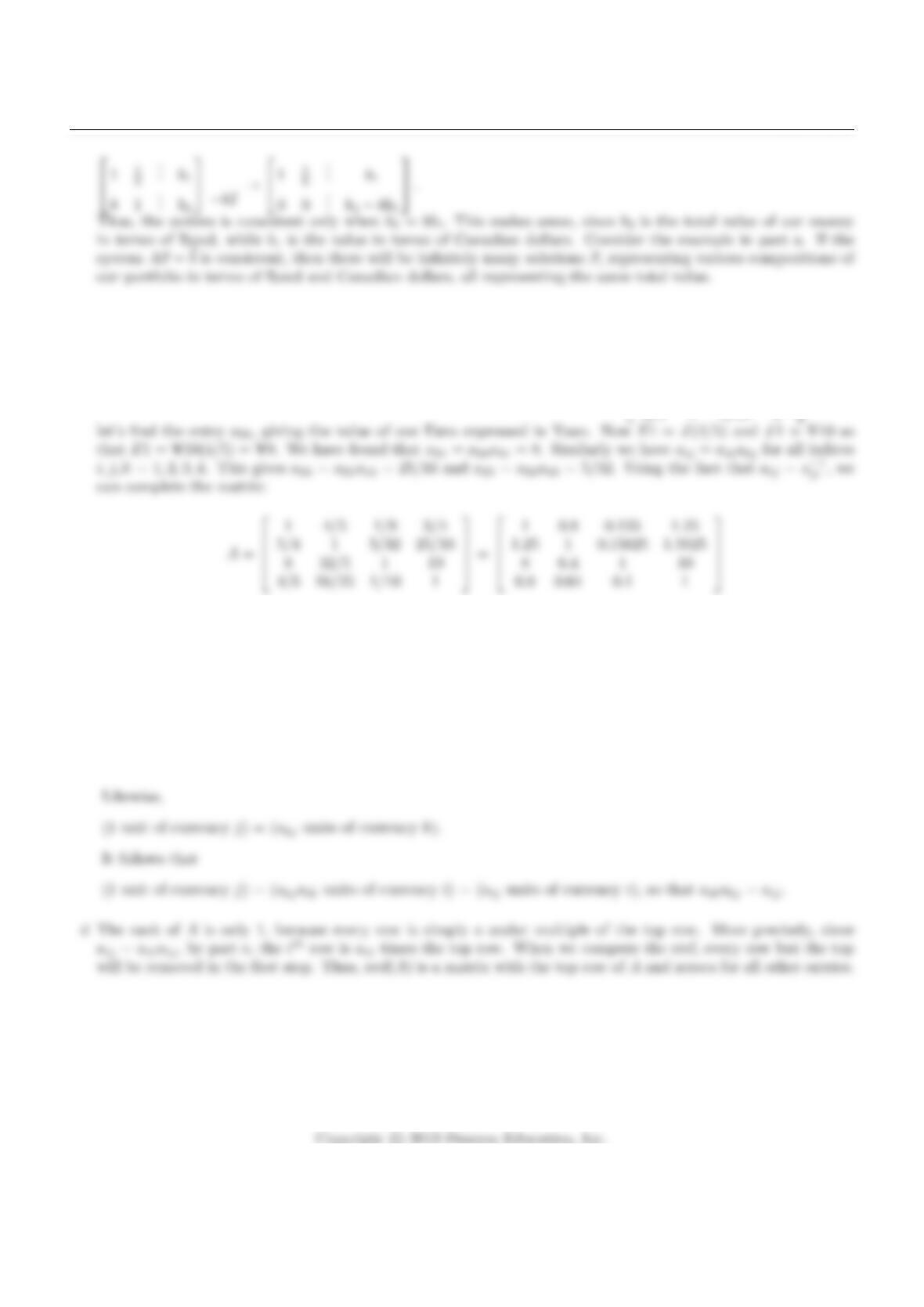
2.1.61 All four entries along the diagonal must be 1: they represent the process of converting a currency to itself.
We also know that aij =a−1
ji for all iand jbecause converting currency ito currency jis the inverse of
converting currency jto currency i. This gives us three more entries, A=
1 4/5∗5/4
5/4 1 ∗ ∗
∗ ∗ 1 10
4/5∗1/10 1
. Next
2.1.62 a 1: this represents converting a currency to itself.
baij is the reciprocal of aji, meaning that aij aji = 1. This represents converting on currency to another, then
converting it back.
c Note that aik is the conversion factor from currency kto currency imeaning that
(1 unit of currency k) = (aik units of currency i)
2.1.63 a We express the leading variables x1, x3, x4in terms of the free variables x2, x5:
x1=x2−4x5
x3=x5
x4= 2x5
65
Chapter 2
2.1.64 a The given system reduces to
x1+2x2+3x4= 0
x3+4x4= 0 or x1=−2x2−3x4
x3=−4x4
Section 2.2
2.2.1The standard L is transformed into a distorted L whose foot is the vector T1
0=3 1
1 2 1
0=3
1.
Meanwhile, the back becomes the vector T0
2=3 1
1 2 0
2=2
4.
2.2.4By Theorem 2.2.4, this is a rotation combined with a scaling. The transformation rotates 45 degrees counter-
clockwise, and has a scaling factor of √2.
2.2.5Note that cos(θ) = −0.8, so that θ= arccos(−0.8) ≈2.498.
66
Section 2.2
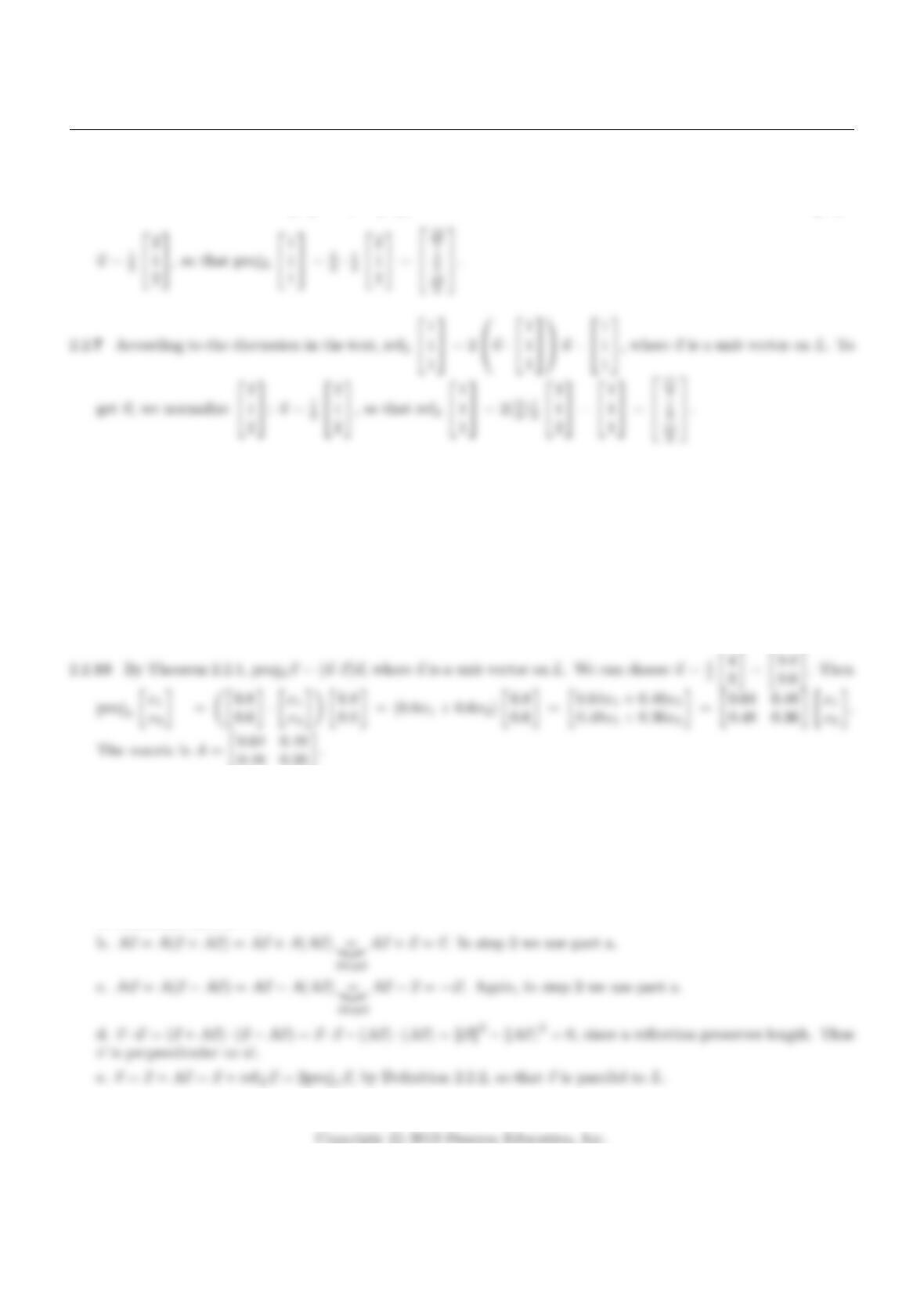
2.2.6By Theorem 2.2.1, projL
1
1
1
=
~u ·
1
1
1
~u, where ~u is a unit vector on L. To get ~u, we normalize
2
1
2
:
2.2.8From Definition 2.2.2, we can see that this is a reflection about the line x1=−x2.
2.2.9By Theorem 2.2.5, this is a vertical shear.
2.2.11 In Exercise 10 we found the matrix A=0.64 0.48
0.48 0.36 of the projection onto the line L. By Theorem 2.2.2,
refL~x = 2(projL~x)−~x = 2A~x −~x = (2A−I2)~x, so that the matrix of the reflection is 2A−I2=0.28 0.96
0.96 −0.28 .
2.2.12 a. If ~x =~xll+~x⊥relative to the line Lof reflection, then A~x =~xll−~x⊥and A(A~x) = ~xll−(−~x⊥) = ~xll+~x⊥=~x.
In summary, A(A~x) = ~x.
67
Chapter 2
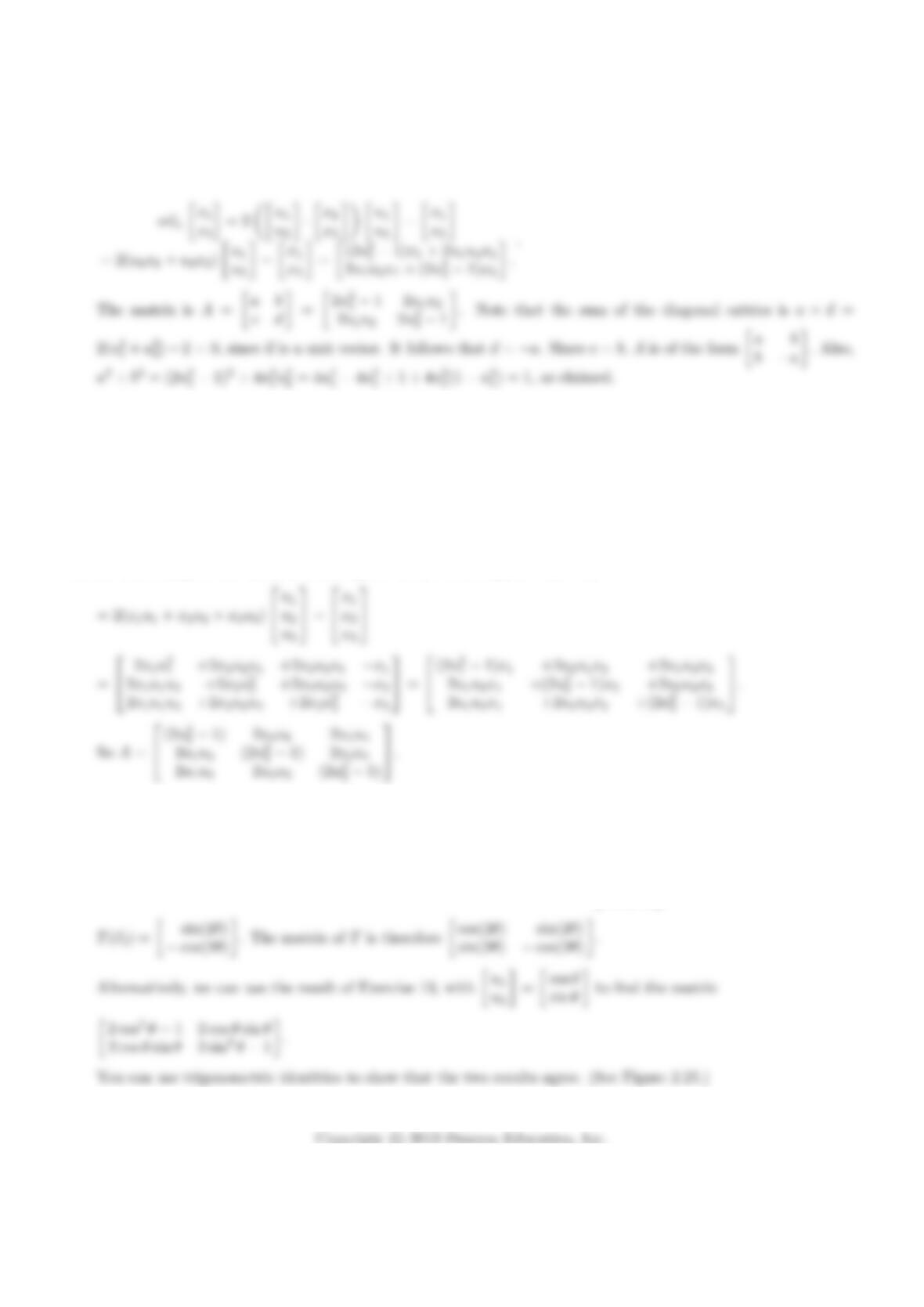
2.2.13 By Theorem 2.2.2,
2.2.14 a Proceeding as on Page 61/62 in the text, we find that Ais the matrix whose ijth entry is uiuj:
A=
u2
1u1u2u1u3
u2u1u2
2u2u3
unu1unu2u2
3
b The sum of the diagonal entries is u2
1+u2
2+u2
3= 1, since ~u is a unit vector.
2.2.15 According to the discussion on Page 60 in the text, refL(~x) = 2(~x ·~u)~u −~x
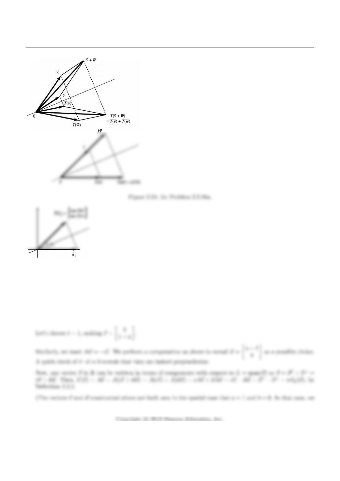
2.2.16 a See Figure 2.24.
b By Theorem 2.1.2, the matrix of Tis [T(~e1)T(~e2)].
T(~e2) is the unit vector in the fourth quadrant perpendicular to T(~e1) = cos(2θ)
sin(2θ), so that
68
Section 2.2
Figure 2.25: for Problem 2.2.16b.
2.2.17 We want, a b
b−av1
v2=av1+bv2
bv1−av2=v1
v2.
Now, (a−1)v1+bv2= 0 and bv1−(a+ 1)v2, which is a system with solutions of the form bt
(1 −a)t, where t
is an arbitrary constant.
69