PROBLEM 2.15
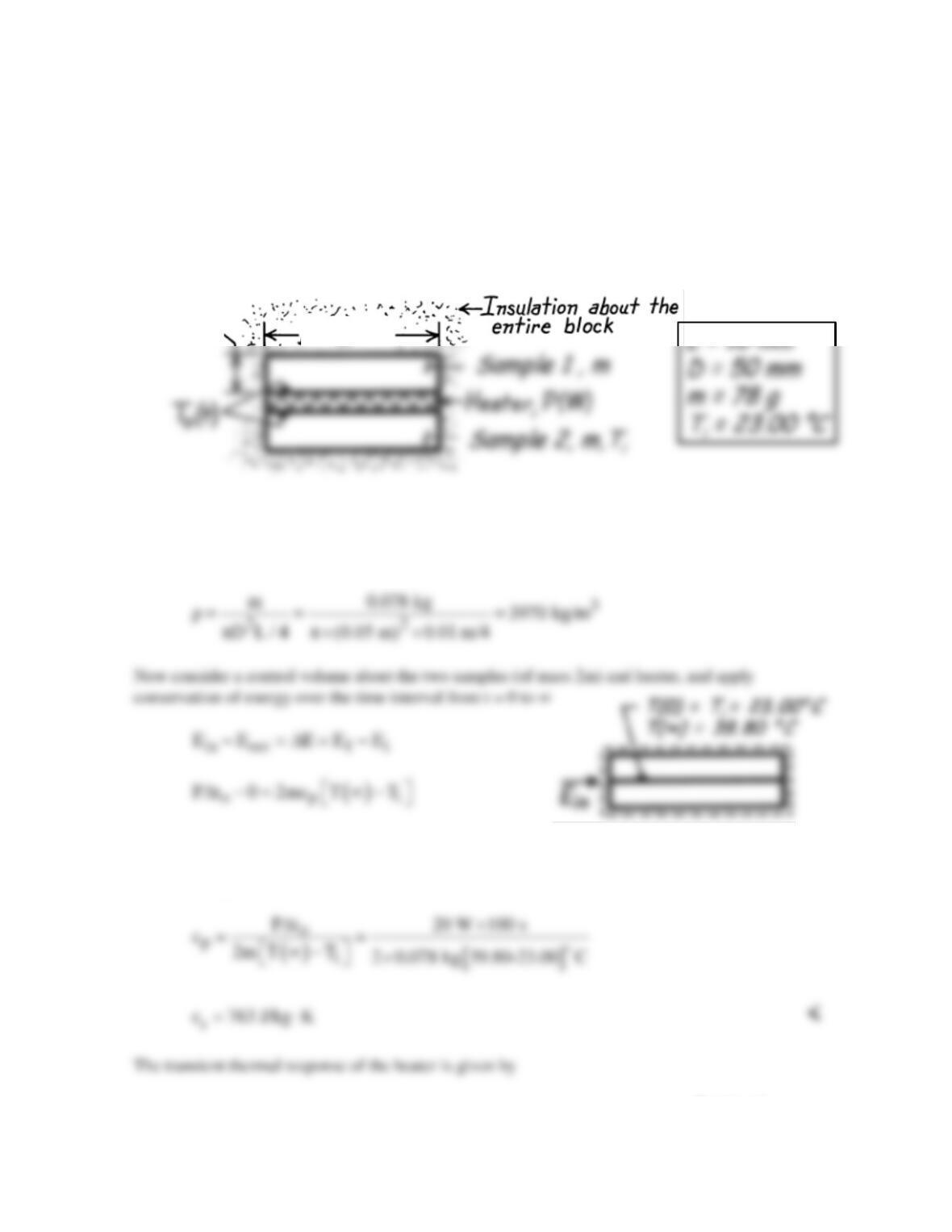
KNOWN: Identical samples of prescribed diameter, length and density initially at a uniform
temperature Ti, sandwich an electric heater which provides a uniform heat flux
′′
qo
for a period of
time ∆to. Conditions shortly after energizing and a long time after de–energizing heater are
prescribed.
FIND: Specific heat and thermal conductivity of the test sample material. From the properties,
identify type of material using Table A.1 or A.2.
SCHEMATIC:
L D
ASSUMPTIONS: (1) One dimensional heat transfer in samples, (2) Constant properties, (3)
Negligible heat loss through insulation, (4) Negligible heater mass.
ANALYSIS: The density of the sample is
where energy inflow is prescribed by the power condition and the final temperature Tf is known.
Solving for cp,
Continued …
PROBLEM 2.15 (Cont.)
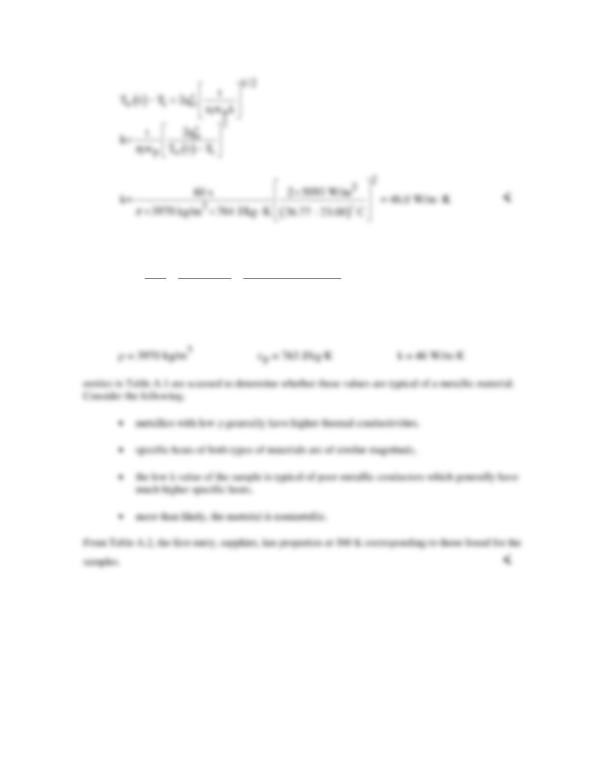
where
()()
2
o2 22
s
P P 20 W
q 5093 W/m .
2A 2 D / 4 2 0.050 / 4 m
ππ
′′ = = = =
×
With the following properties now known,
PROBLEM 2.16
KNOWN: Five materials at 300 K.
FIND: Heat capacity,
ρ
cp. Which material has highest thermal energy storage per unit volume.
Which has lowest cost per unit heat capacity.
ANALYSIS: The values of heat capacity,
ρ
cp, are tabulated below.
Material
Common
brick
Plain carbon
steel
Engine oil
Water
Soil
Heat Capacity
(kJ/m
3
⋅K)
1603
3409
1688
4166
3772
<
Thermal energy storage refers to either sensible or latent energy. The change in sensible energy per
Various materials also have the potential for latent energy storage due to either a solid–liquid or liquid–
vapor phase change. Taking water as an example, the latent heat of fusion is
333.7 kJ/kg. With a density of
ρ
≈ 1000 kg/m3 at 0°C, the latent energy per unit volume associated
with the solid–liquid phase transition is 333,700 kJ/m3. This corresponds to an 80°C temperature
change in the liquid phase. The latent heat of vaporization for water is very large, 2257 kJ/kg, but it is
generally inconvenient to use a liquid–vapor phase change for thermal energy storage because of the
large volume change.
PROBLEM 2.17
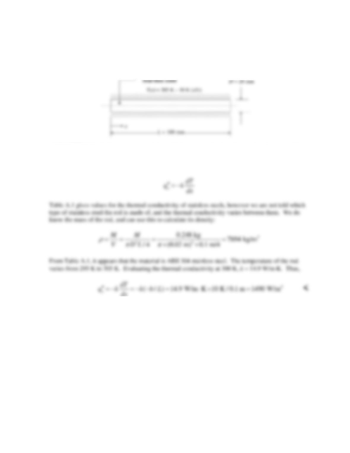
KNOWN: Diameter, length, and mass of stainless steel rod, insulated on its exterior surface other
than ends. Temperature distribution.
FIND: Heat flux.
SCHEMATIC:
ASSUMPTIONS: (1) Steady–state conditions, (2) One–dimensional conduction in x–direction, (3)
Constant properties.
ANALYSIS: The heat flux can be found from Fourier’s law,
COMMENTS: If the temperature of the rod varies significantly along its length, the thermal
conductivity will vary along the rod as much or more than the variation in thermal conductivities
between the different stainless steels.
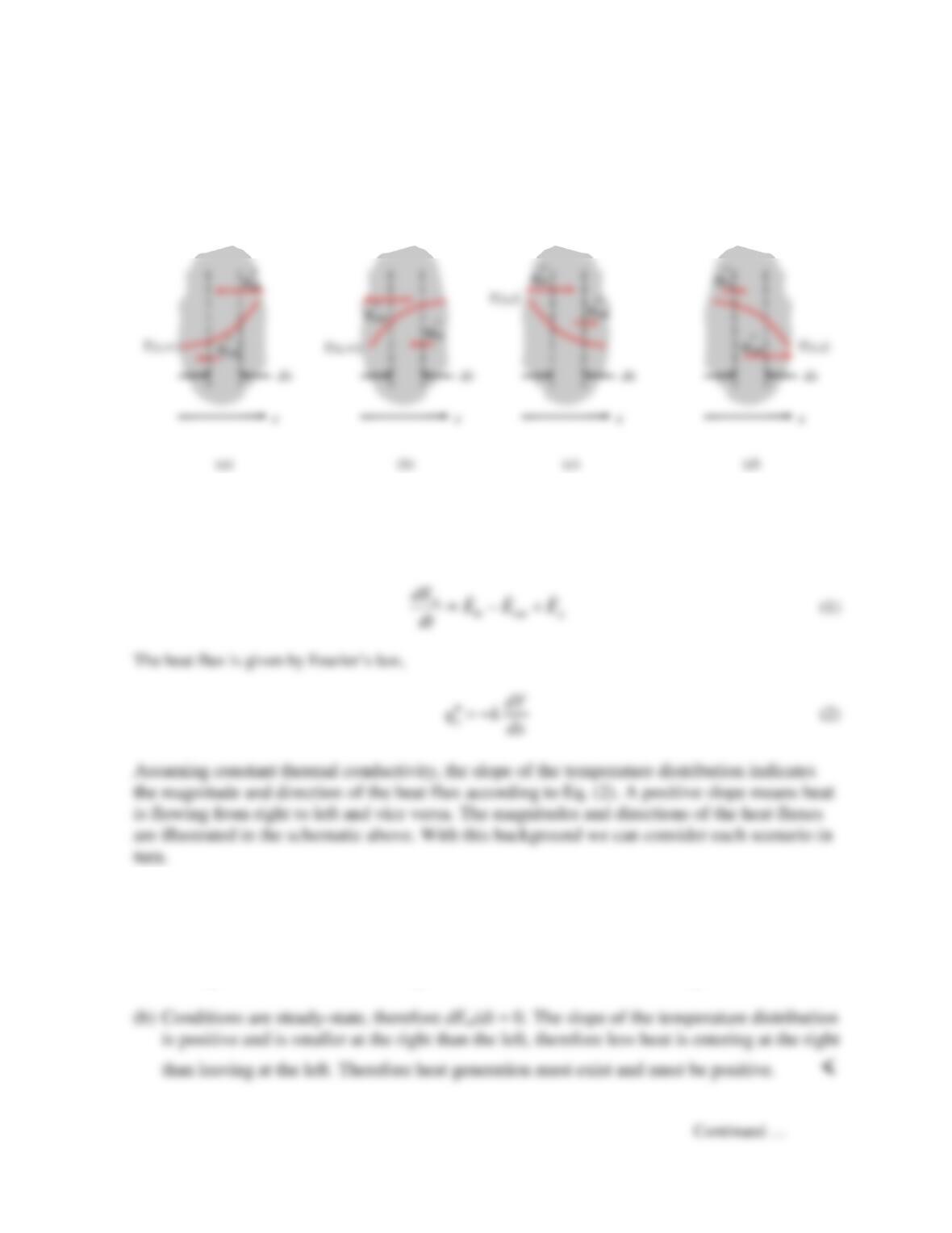
PROBLEM 2.18
KNOWN: Temperature distribution in a plane wall. Whether conditions are steady–state or transient.
FIND: (a) Whether thermal energy is being generated within the wall, and if so, whether it is positive
or negative. (b) Whether the volumetric generation rate is positive or negative. (c) and (d) Whether the
temperature is increasing or decreasing with time.
SCHEMATIC:
ASSUMPTIONS: (1) One–dimensional conduction in x–direction, (2) Constant properties.
ANALYSIS: An energy balance on the differential control volume can be expressed as
(a) Conditions are steady-state, therefore dEst/dt = 0 in Eq. (1). Since the slope of the
temperature distribution is positive, heat is flowing from right to left in the schematic.
With the slope higher at the right than the left, more heat is entering at the right than
leaving at the left. Therefore heat generation must exist and must be negative. <
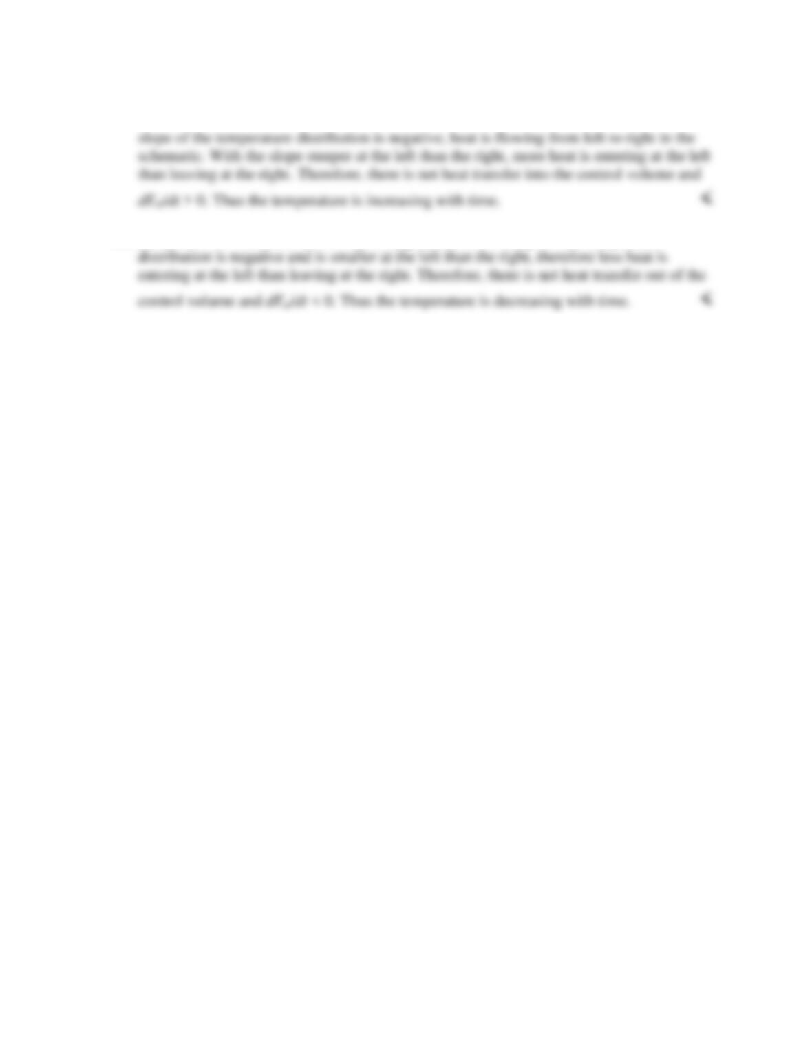
PROBLEM 2.18 (Cont.)
(c) Conditions are transient. There is no heat generation, therefore
0
g
E=
in Eq. (1). Since the
(d) Conditions are transient. There is no heat generation. The slope of the temperature
COMMENTS: If the thermal conductivity is not constant, it is not possible to tell whether the heat
flux is higher or lower at the two sides of the control volume.
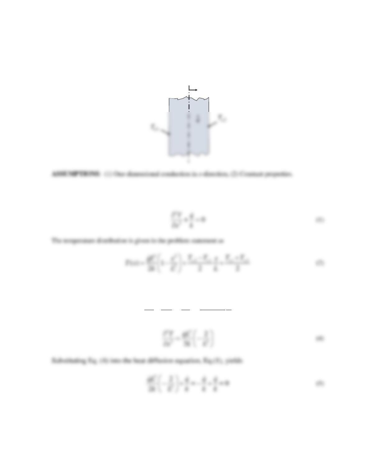
PROBLEM 2.19
KNOWN: Temperature distribution in a plane wall experiencing uniform volumetric heat generation.
FIND: Whether the steady-state form of the heat diffusion equation is satisfied. Expression for the
heat flux distribution.
SCHEMATIC:
-L +L
x
ANALYSIS: The heat diffusion equation with constant properties is given by Eq. 2.21. Under one-
dimensional, steady-state conditions this reduces to
This temperature distribution can be substituted into Eq. (1) to see if it is satisfied. Taking the
derivative of Eq. (2) twice,
2
,2 ,1
2
21
22
ss
TT
T qL x
x kL L
−
∂
= −+
∂
(3)
Therefore the steady-state form of the heat diffusion equation is satisfied. <
Continued …
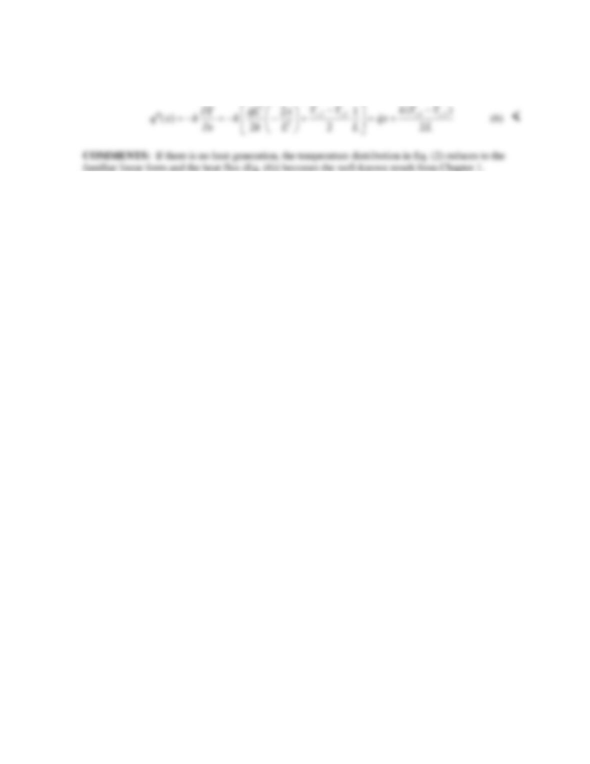
PROBLEM 2.19 (Cont.)
The heat flux is given by Fourier’s Law, with the temperature derivative from Eq. (3).
Therefore,
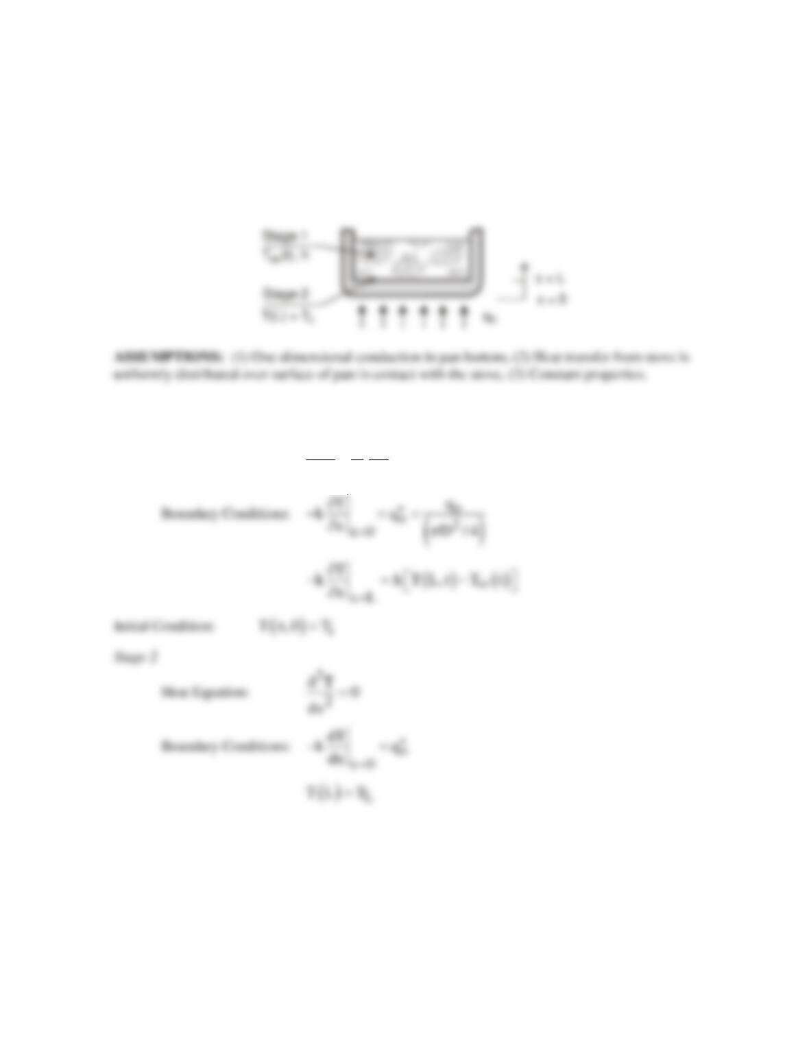
PROBLEM 2.20
KNOWN: Diameter D, thickness L and initial temperature Ti of pan. Heat rate from stove to bottom
of pan. Convection coefficient h and variation of water temperature T∞(t) during Stage 1.
Temperature TL of pan surface in contact with water during Stage 2.
FIND: Form of heat equation and boundary conditions associated with the two stages.
SCHEMATIC:
ANALYSIS:
Stage 1
Heat Equation:
2
2
T 1T
t
x
α
∂∂
=∂
∂
COMMENTS: Stage 1 is a transient process for which T∞(t) must be determined separately. As a
first approximation, it could be estimated by neglecting changes in thermal energy storage by the pan
bottom and assuming that all of the heat transferred from the stove acted to increase thermal energy
storage within the water. Hence, with q ≈ mcp dT∞/dt, where m and cp are the mass and specific heat
of the water in the pan, T∞(t) ≈ (q/mcp) t.
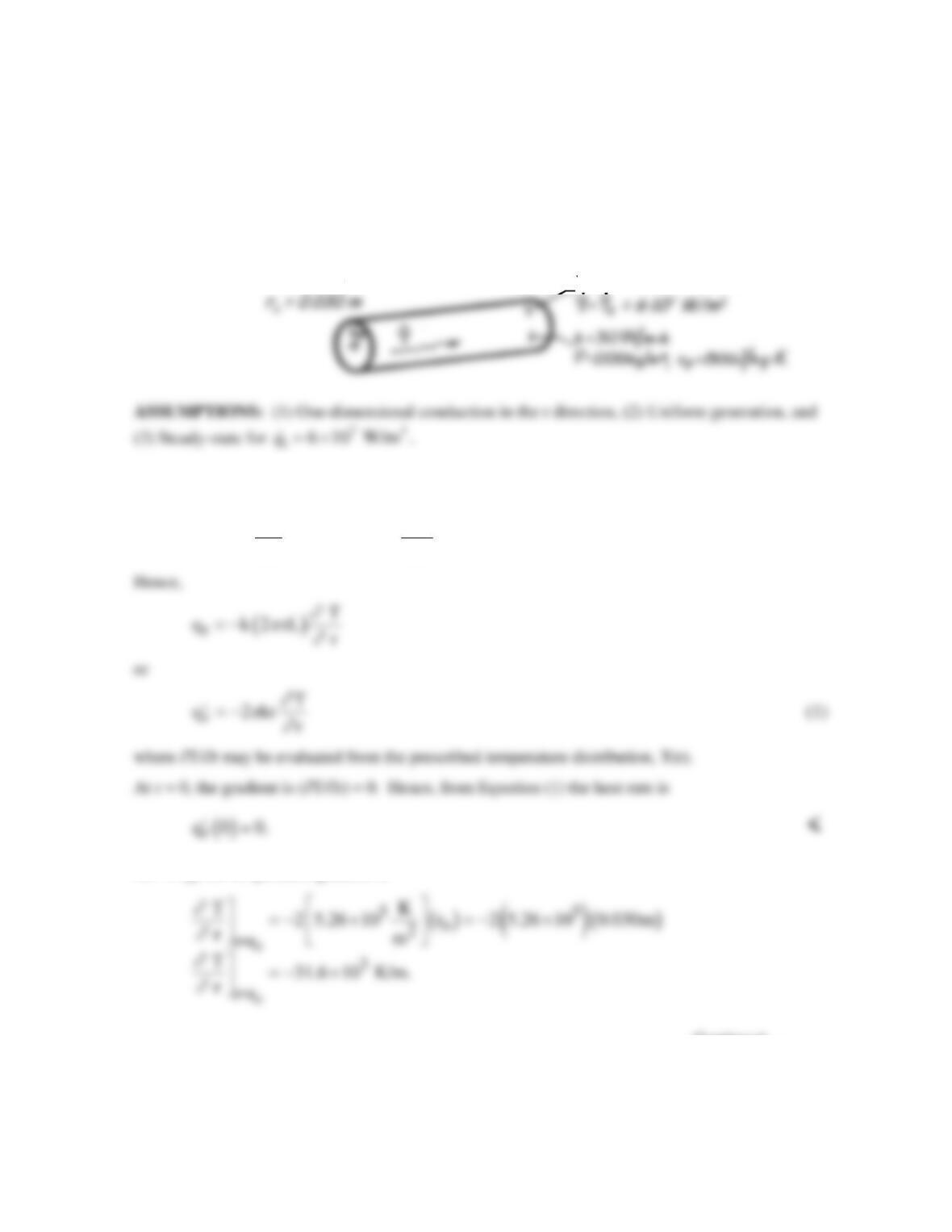
PROBLEM 2.21
KNOWN: Steady–state temperature distribution in a cylindrical rod having uniform heat generation
of
73
1
6 10 W/mq= ×
.
FIND: (a) Steady–state centerline and surface heat transfer rates per unit length,
′
q
r
.
(b) Initial time
rate of change of the centerline and surface temperatures in response to a change in the generation rate
from
83
12
q to q = 10 W/m .
SCHEMATIC:
ANALYSIS: (a) From the rate equations for cylindrical coordinates,
′′ = −q k T
r q = -kA T
r
r r
∂
∂
∂
∂
.
At r = ro, the temperature gradient is
Continued …
T(r) = 900 –5.26∙10
5
r
2
PROBLEM 2.21 (Cont.)
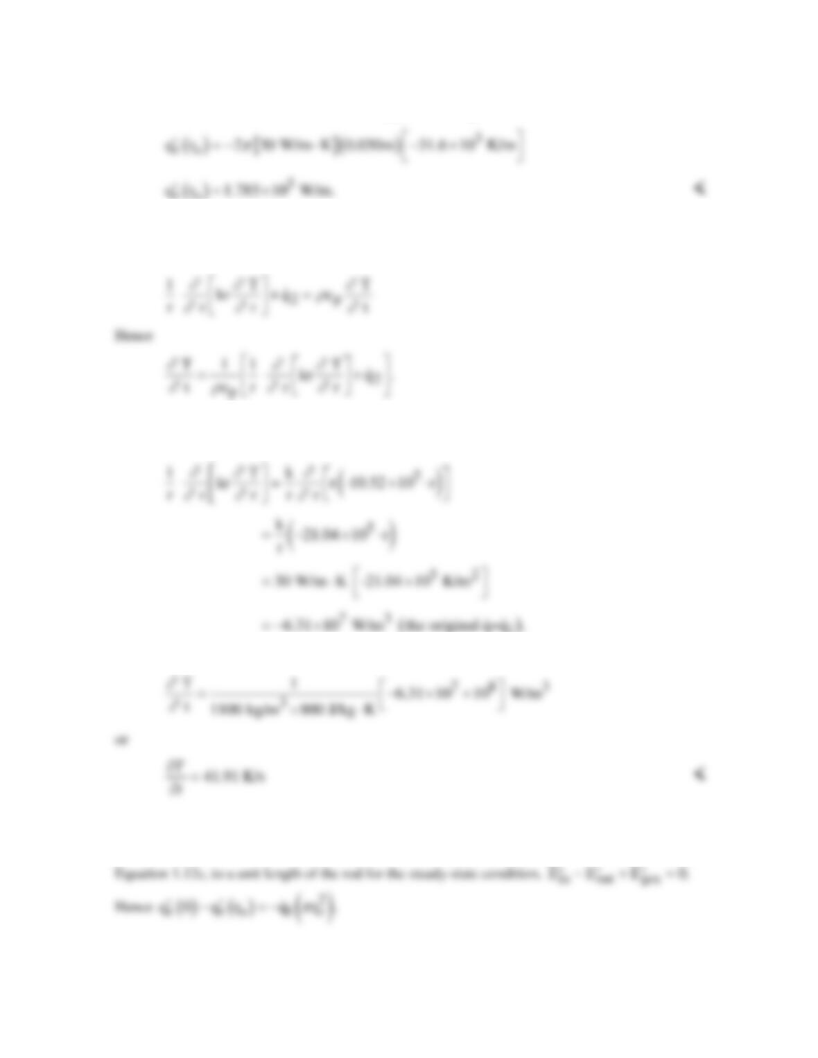
Hence, the heat rate at the outer surface (r = ro) per unit length is
ro
(b) Transient (time–dependent) conditions will exist when the generation is changed, and for the
prescribed assumptions, the temperature is determined by the following form of the heat equation,
Equation 2.26
However, initially (at t = 0), the temperature distribution is given by the prescribed form, T(r) = 800 –
5.26×10⁵r2, and
Hence, everywhere in the wall,
COMMENTS: (1) The value of (∂T/∂t) will decrease with increasing time, until a new steady–state
condition is reached and once again (∂T/∂t) = 0. (2) By applying the energy conservation requirement,
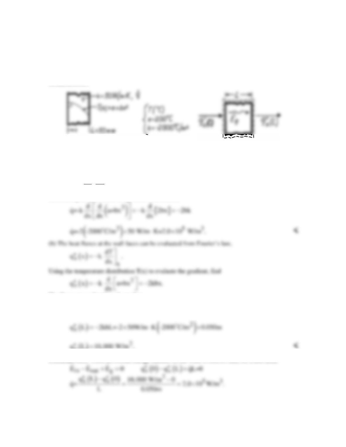
PROBLEM 2.22
KNOWN: Temperature distribution in a one-dimensional wall with prescribed thickness and thermal
conductivity.
FIND: (a) The heat generation rate,
q,
in the wall, (b) Heat fluxes at the wall faces and relation to
q.
SCHEMATIC:
ASSUMPTIONS: (1) Steady-state conditions, (2) One-dimensional heat flow, (3) Constant
properties.
ANALYSIS: (a) The appropriate form of the heat equation for steady-state, one-dimensional
conditions with constant properties is Eq. 2.21 re–written as
d dT
q=-k dx dx
Substituting the prescribed temperature distribution,
The fluxes at x = 0 and x = L are then
(
)
x
q0 0
′′ =
<
( )
x
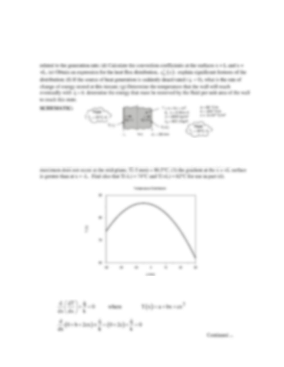
COMMENTS: From an overall energy balance on the wall, it follows that, for a unit area,
PROBLEM 2.23
KNOWN: Analytical expression for the steady-state temperature distribution of a plane wall
experiencing uniform volumetric heat generation
q
while convection occurs at both of its surfaces.
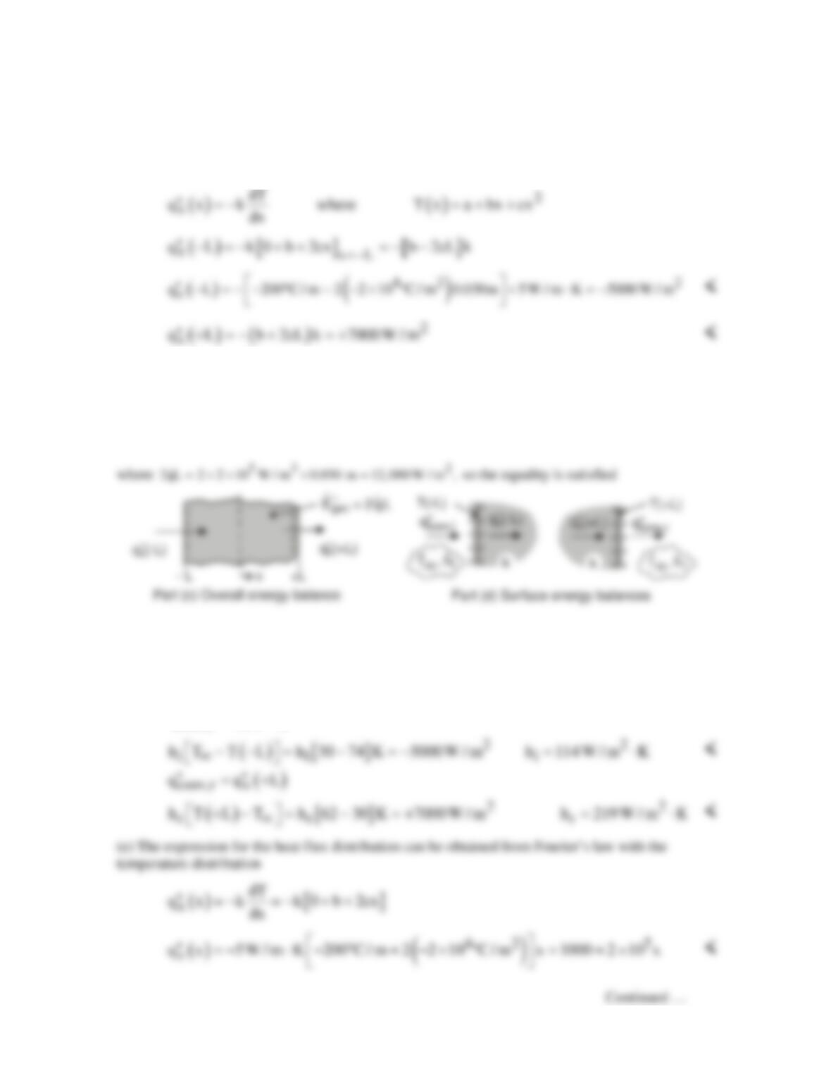
FIND: (a) Sketch the temperature distribution, T(x), and identify significant physical features, (b)
Determine
q
, (c) Determine the surface heat fluxes,
( )
x
qL
′′ −
and
( )
x
q L;
′′ +
how are these fluxes
ASSUMPTIONS: (1) Steady–state conditions, (2) Uniform volumetric heat generation, (3) Constant
properties.
ANALYSIS: (a) Using the analytical expression in the Workspace of IHT, the temperature
distribution appears as shown below. The significant features include (1) parabolic shape, (2)
(b) Substituting the temperature distribution expression into the appropriate form of the heat diffusion
equation, Eq. 2.21, the rate of volumetric heat generation can be determined.
x
q
PROBLEM 2.23 (Cont.)
()
42 5 3
q 2ck 2 2 10 C / m 5W / m K 2 10 W / m=− =− −× ° ⋅ = ×
<
(c) The heat fluxes at the two boundaries can be determined using Fourier’s law and the temperature
distribution expression.
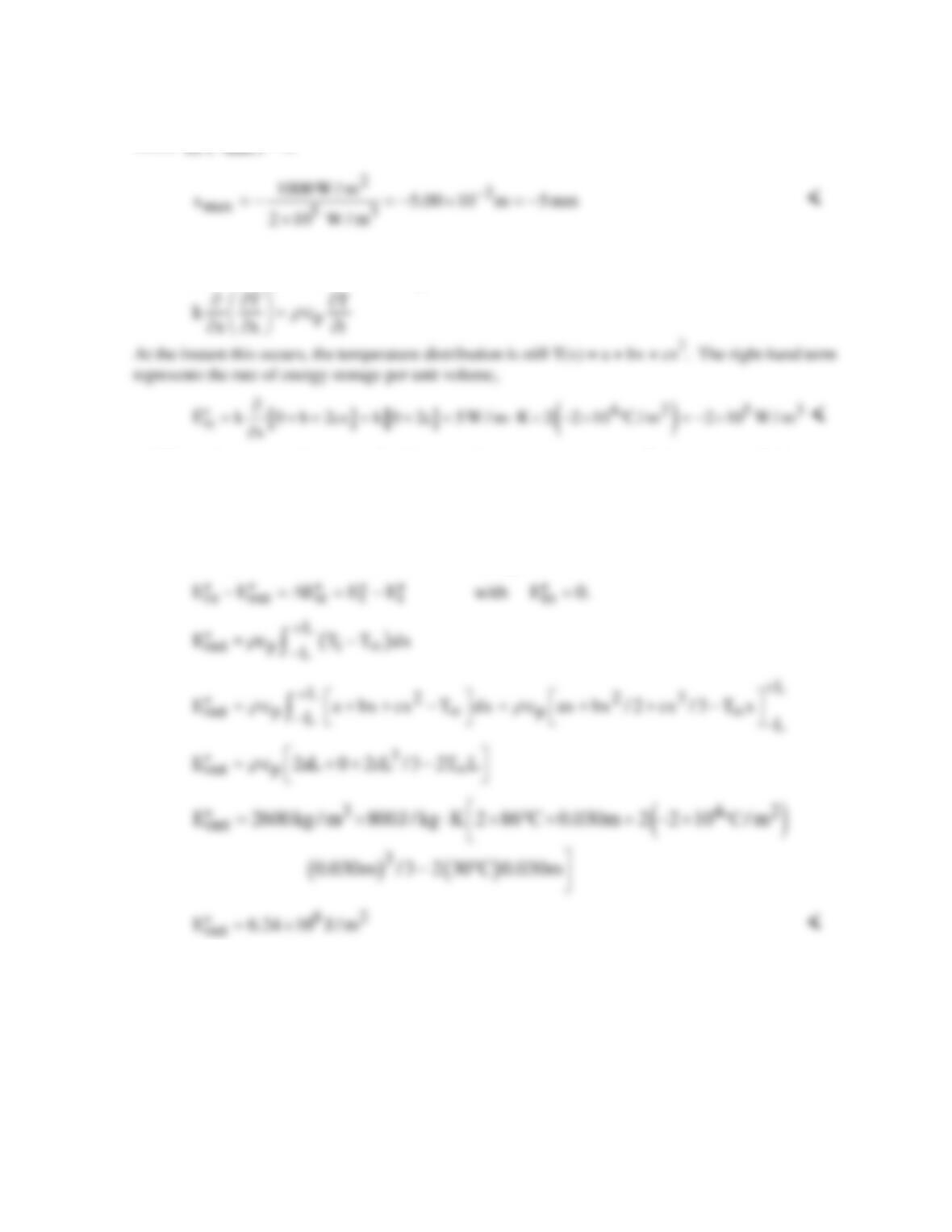
From an overall energy balance on the wall as shown in the sketch below,
in out gen
E E E 0,−+ =
( ) ( )
?22 2
xx
q L q L 2qL 0 or 5000 W / m 7000 W / m 12,000 W / m 0
′′ ′′
+ −− ++ = − − + =
(d) The convection coefficients, hl and hr, for the left– and right-hand boundaries (x = –L and x= +L,
respectively), can be determined from the convection heat fluxes that are equal to the conduction
fluxes at the boundaries. See the surface energy balances in the sketch above. See also part (a) result
for T(–L) and T(+L).
( )
conv, x
q qL
′′ ′′
= −
PROBLEM 2.23 (Cont.)
The distribution is linear with the x-coordinate. The maximum temperature will occur at the location
where
( )
q x 0,
′′ =
(f) If the source of the heat generation is suddenly deactivated so that
q
= 0, the appropriate form of
the heat diffusion equation for the ensuing transient conduction is
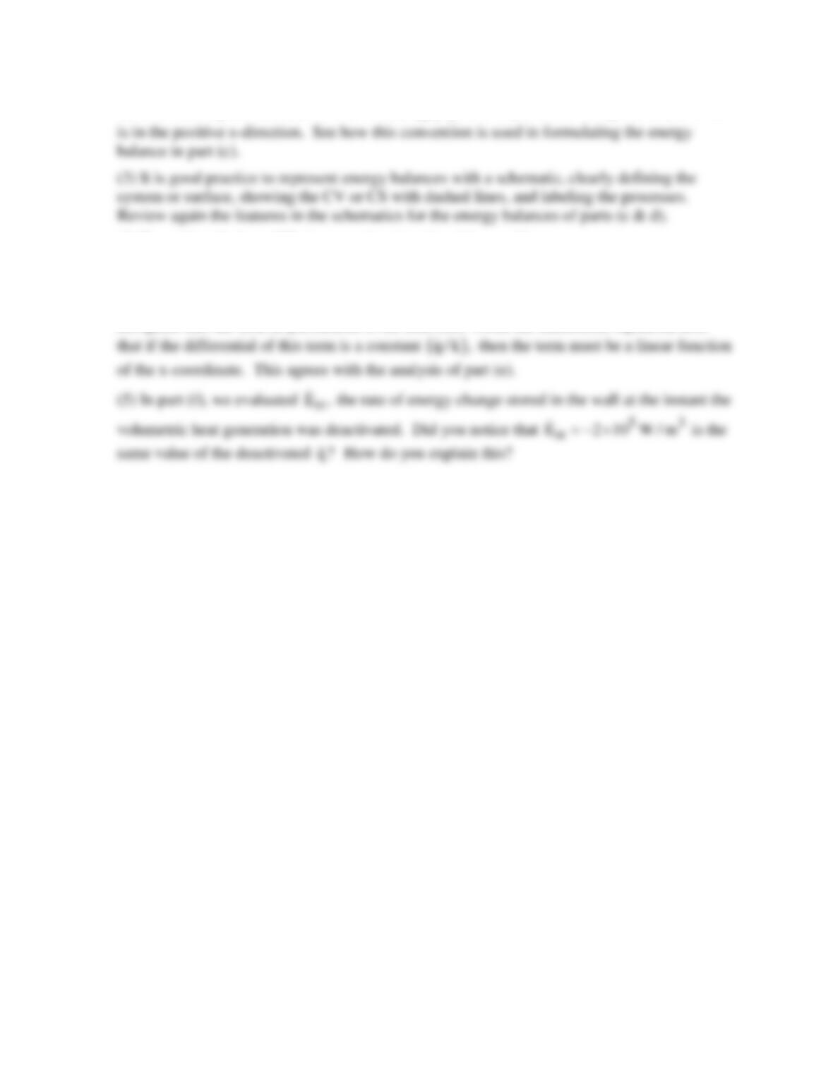
(g) With no heat generation, the wall will eventually (t → ∞) come to equilibrium with the fluid,
T(x,∞) = T∞ = 30°C. To determine the energy that must be removed from the wall to reach this state,
apply the conservation of energy requirement over an interval basis, Eq. 1.12b. The “initial” state is
that corresponding to the steady-state temperature distribution, Ti, and the “final” state has Tf = 30°C.
We’ve used T∞ as the reference condition for the energy terms.
COMMENTS: (1) In part (a), note that the temperature gradient is larger at x = + L than at x
= – L. This is consistent with the results of part (c) in which the conduction heat fluxes are
evaluated.
Continued …
PROBLEM 2.23 (Cont.)
(2) In evaluating the conduction heat fluxes,
( )
x
q x,
′′
it is important to recognize that this flux
(4) Re–writing the heat diffusion equation introduced in part (b) as
d dT
k q0
dx dx
− − +=
recognize that the term in parenthesis is the heat flux. From the differential equation, note
PROBLEM 2.24
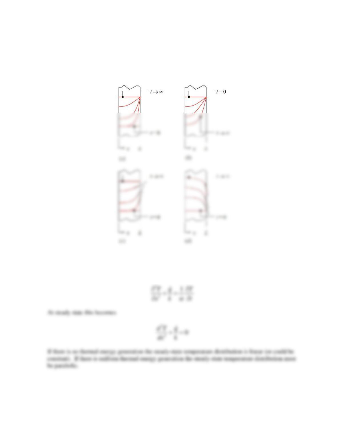
KNOWN: Transient temperature distributions in a plane wall.
FIND: Appropriate forms of heat equation, initial condition, and boundary conditions.
SCHEMATIC:
ASSUMPTIONS: (1) One–dimensional conduction, (2) Constant properties, (3) Negligible radiation.
ANALYSIS: The general form of the heat equation in Cartesian coordinates for constant k is
Equation 2.21. For one-dimensional conduction it reduces to
Continued…
PROBLEM 2.24 (Cont.)
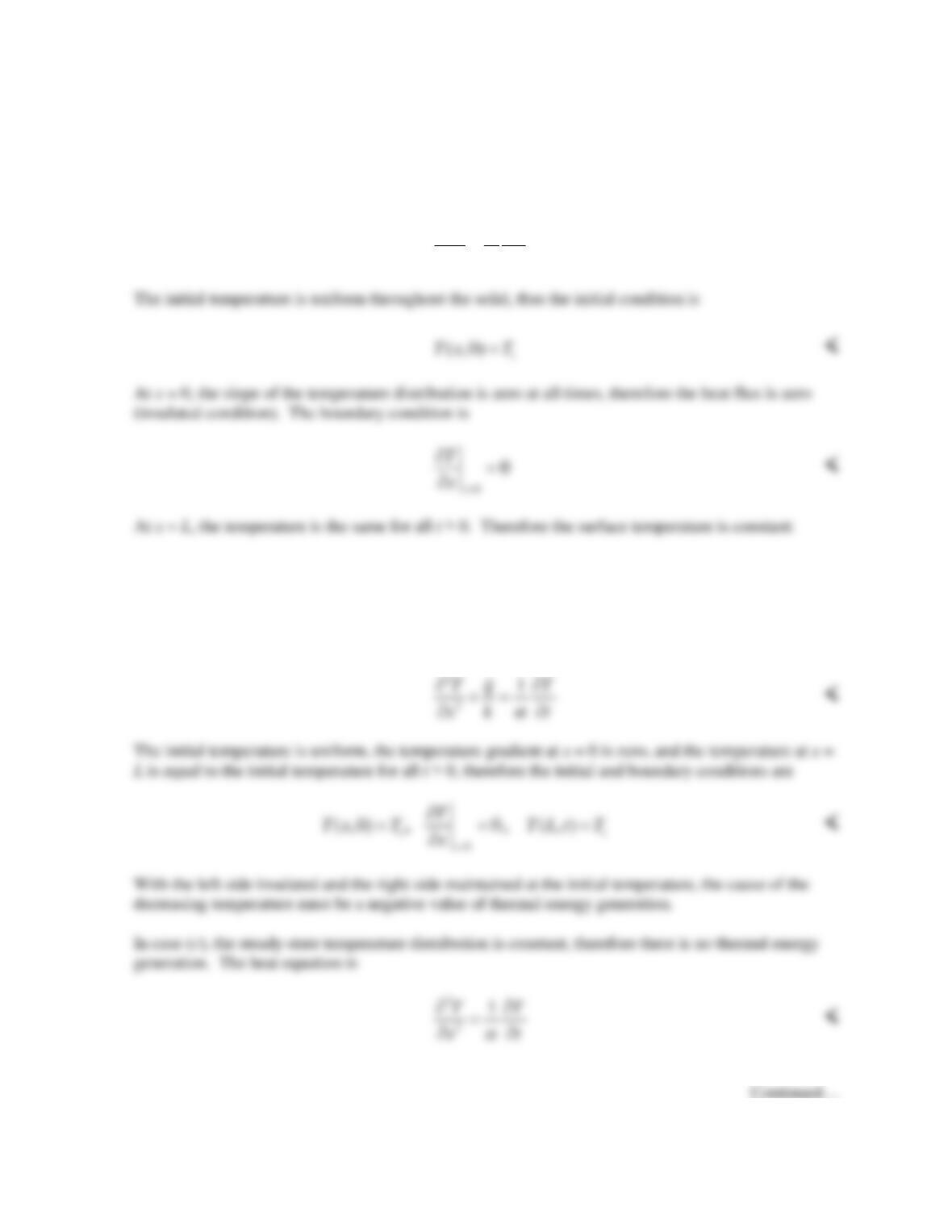
In case (a), the steady–state temperature distribution is constant, therefore there must not be any
thermal energy generation. The heat equation is
2
2
1
TT
xt
α
∂∂
=
∂∂
<
( ,) s
T Lt T=
<
For case (b), the steady-state temperature distribution is not linear and appears to be parabolic,
therefore there is thermal energy generation. The heat equation is
α
∂∂
PROBLEM 2.24 (Cont.)
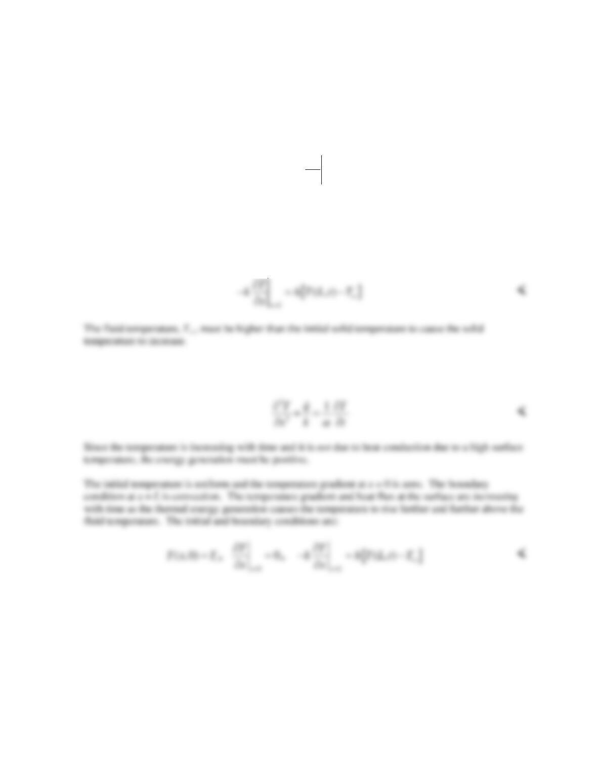
The initial temperature is uniform throughout the solid. At x = 0, the slope of the temperature
distribution is zero at all times. Therefore the initial condition and boundary condition at x = 0 are
( ,0) i
Tx T=
,
0
0
x
T
x
=
∂=
∂
<
At x = L, neither the temperature nor the temperature gradient are constant for all time. Instead, the
temperature gradient is decreasing with time as the temperature approaches the steady–state
temperature. This corresponds to a convection heat transfer boundary condition. As the surface
temperature approaches the fluid temperature, the heat flux at the surface decreases. The boundary
condition is:
For case (d), the steady–state temperature distribution is not linear and appears to be parabolic,
therefore there is thermal energy generation. The heat equation is
Tx T=
COMMENTS: 1. You will learn to solve for the temperature distribution in transient conduction in
Chapter 5. 2. Case (b) might correspond to a situation involving a spatially-uniform endothermic
chemical reaction. Such situations, although they can occur, are not common.
PROBLEM 2.25
KNOWN: Rod consisting of two materials with same lengths. Ratio of thermal conductivities.
FIND: Sketch temperature and heat flux distributions.
SCHEMATIC:
ASSUMPTIONS: (1) Steady–state conditions, (2) One–dimensional conduction, (3) Constant
properties, (3) No internal generation.
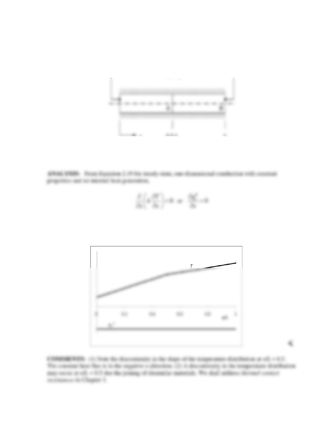
From these equations we know that heat flux is constant and the temperature gradient is inversely
proportional to k. Thus, with kA = 0.5kB, we can sketch the temperature and heat flux distributions as
shown below:
x L
T1T2
T1 < T2
0.5 L