CHAPTER 2 │ DESCRIPTIVE STATISTICS 55
b.
Salary, x
(1000s of dollars)
Deviation, x – µ
(100s of dollars)
23 –18.5
29 –12.5
32 –9.5
40 –1.5
3ab. 41.5µ=, or $41,500
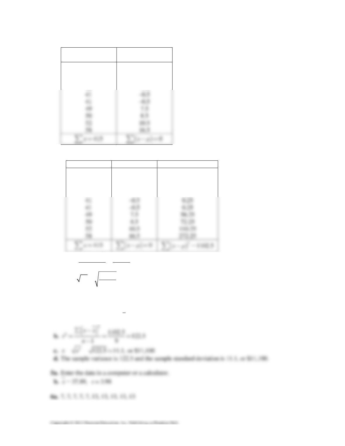
Salary, x x – µ (x – µ)2
23 –18.5 342.25
29 –12.5 156.25
32 –9.5 90.25
40 –1.5 2.25
c.
()
2
21102.5 110.3
10
x
N
µ
σ∑−
==≈
d. 21102.5 10.5,
10
σσ== = or $10,500
e. The population variance is about 110.3 and the population standard deviation is 10.5, or
$10,500.
4a. From 3ab,
()
21102.5.
x
SS x x=∑ − =
56 CHAPTER 2 │ DESCRIPTIVE STATISTICS
b.
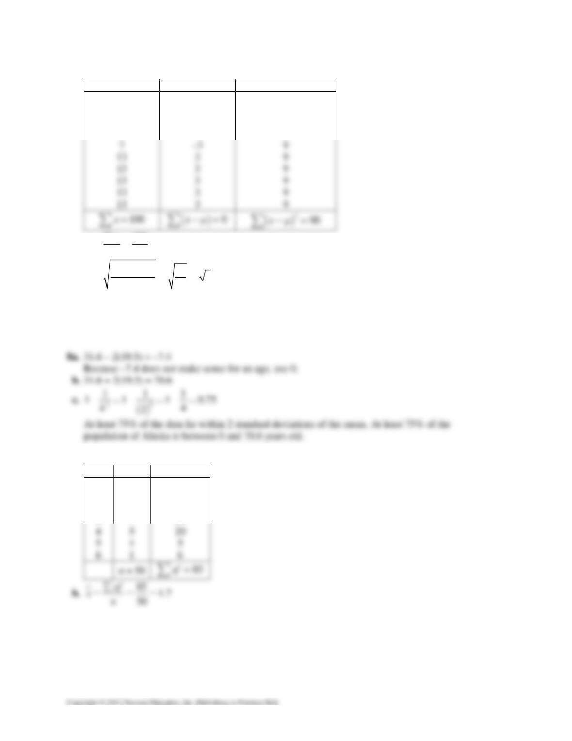
Salary, x x – µ (x – µ)2
7 –3 9
7 –3 9
7 –3 9
7 –3 9
100 10
10
x
N
µ∑
===
()
290 93
10
x
N
µ
σ∑−
====
7a. 66.92 – 64.3 = 2.62 = 1 standard deviation
b. 34%
c. Approximately 34% of women ages 20-29 are between 64.3 and 66.92 inches tall.
9a.
x f xf
0 10 0
1 19 19
2 7 14
3 7 21
CHAPTER 2 │ DESCRIPTIVE STATISTICS 57
c.
−
x
x
()
−2
x
x
()
−2
x
xf
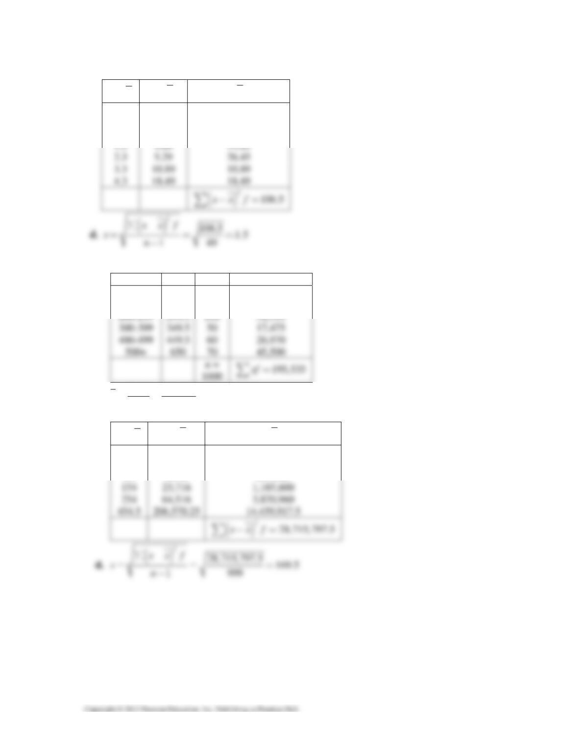
–1.7 2.89 28.90
–0.7 0.49 9.31
0.3 0.09 0.63
10a.
Class x f xf
1-99 49.5 380 18,810
100-199 149.5 230 34,385
b. 195,535 195.5
1000
xf
xn
∑
== ≈
c.
−
x
x
()
−2
x
x
()
−2
x
xf
–146 21,316 8,100,080
–46 2116 486,680
54 2916 612,360
2.4 EXERCISE SOLUTIONS
1. The range is the difference between the maximum and minimum values of a data set. The
advantage of the range is that it is easy to calculate. The disadvantage is that it uses only two
entries from the data set.
58 CHAPTER 2 │ DESCRIPTIVE STATISTICS
2. A deviation
()
xµ− is the difference between an entry x and the mean of the data µ. The sum of
the deviations is always zero.
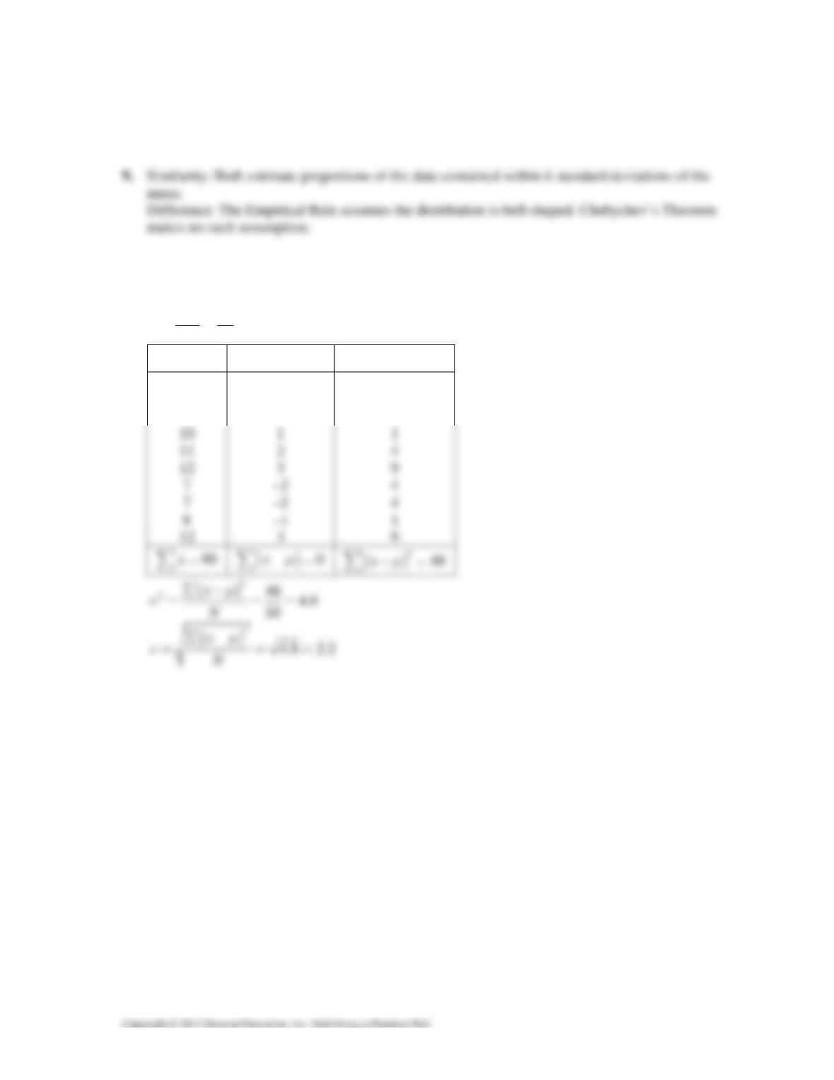
5. {9, 9, 9, 9, 9, 9, 9}
n = 7
63 9
7
x
xn
∑
===
x
−
x
x
()
−2
x
x
9 0 0
9 0 0
9 0 0
6. {3, 3, 3, 7, 7, 7}
n = 6
30 5
6
x
n
µ∑
===
x
−
x
µ
()
−2
xµ
3 –2 4
3 –2 4
3 –2 4
7. When calculating the population standard deviation, you divide the sum of the squared deviations
by N, then take the square root of that value. When calculating the sample standard deviation, you
divide the sum of the squared deviations by 1n−, then take the square root of that value.
CHAPTER 2 │ DESCRIPTIVE STATISTICS 59
8. When given a data set one would have to determine if it represented the population or if it was a
sample taken from the population. If the data are a population, then σ is calculated. If the data
are a sample, then s is calculated.
10. You must know that the distribution is bell-shaped.
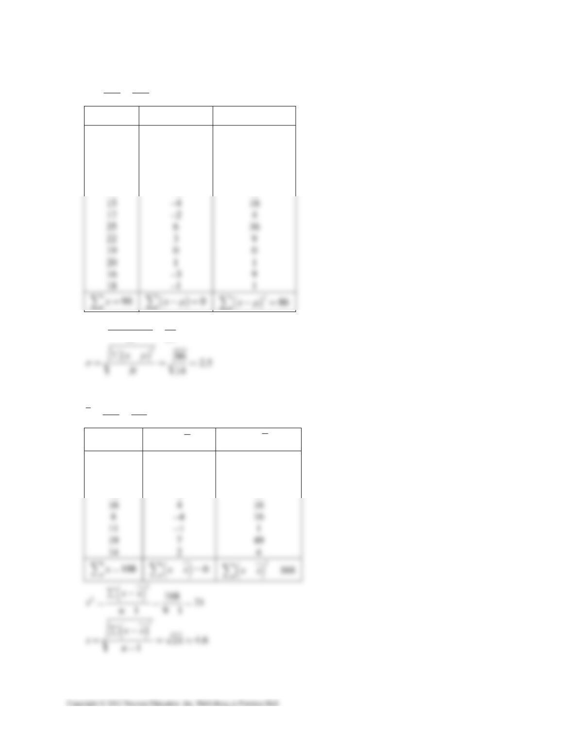
11. Range = Max – Min = 12 – 5 = 7
90 9
10
x
N
µ∑
===
x
−
x
µ
()
−2
xµ
9 0 0
5 –4 16
9 0 0
60 CHAPTER 2 │ DESCRIPTIVE STATISTICS
12. Range = Max – Min = 25 – 15 = 10
266 19
14
x
N
µ∑
===
x
−
x
µ
()
−2
xµ
18 –1 1
20 1 1
19 0 0
21 2 4
19 0 0
17 –2 4
()
2
286 6.1
14
x
N
µ
σ∑−
==≈
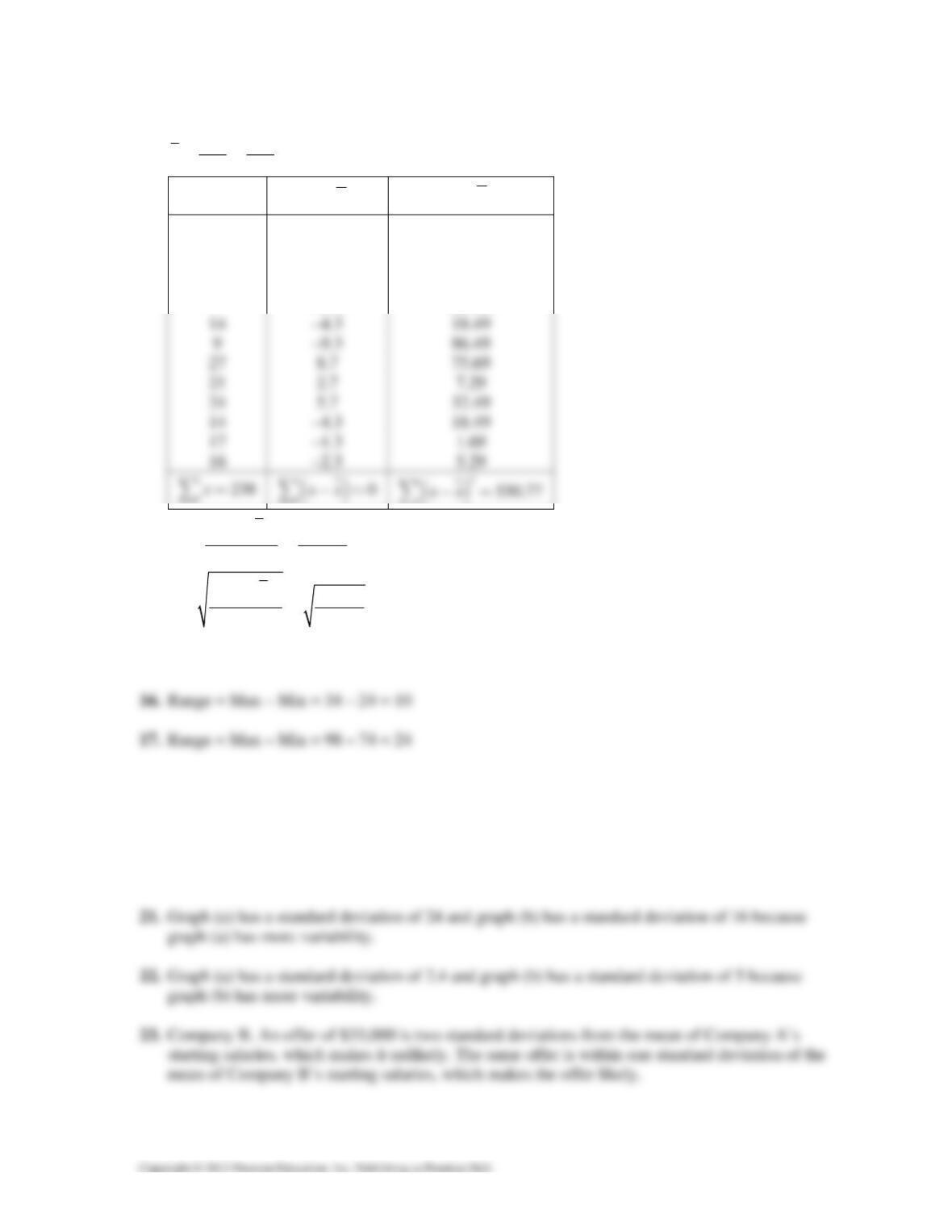
13. Range = Max – Min = 19 – 4 = 15
108 12
9
x
xn
∑
===
x
−
x
x
()
−2
x
x
4 –8 64
15 3 9
9 –3 9
12 0 0
CHAPTER 2 │ DESCRIPTIVE STATISTICS 61
14. Range = Max – Min = 28 – 7 = 21
238 18.3
13
x
xn
∑
==≈
x
−
x
x
()
−2
x
x
28 9.7 94.09
25 6.7 44.89
21 2.7 7.29
15 –3.3 10.89
7 –11.3 127.69
()
2
2530.77 44.2
1131
xx
sn
∑−
==≈
−−
()
2
530.77 6.7
112
xx
sn
∑−
==≈
−
15. Range = Max – Min = 96 – 23 = 73
18. Range = Max – Min = 6.7 – 0.5 = 6.2
19a. Range = Max – Min = 38.5 – 20.7 = 17.8
b. Range = Max – Min = 60.5 – 20.7 = 39.8
20. Changing the maximum value of the data set greatly affects the range.
62 CHAPTER 2 │ DESCRIPTIVE STATISTICS
24. Player B. A smaller standard deviation means that Player B’s scores tend to fall within a smaller
interval of values than Player A’s scores.
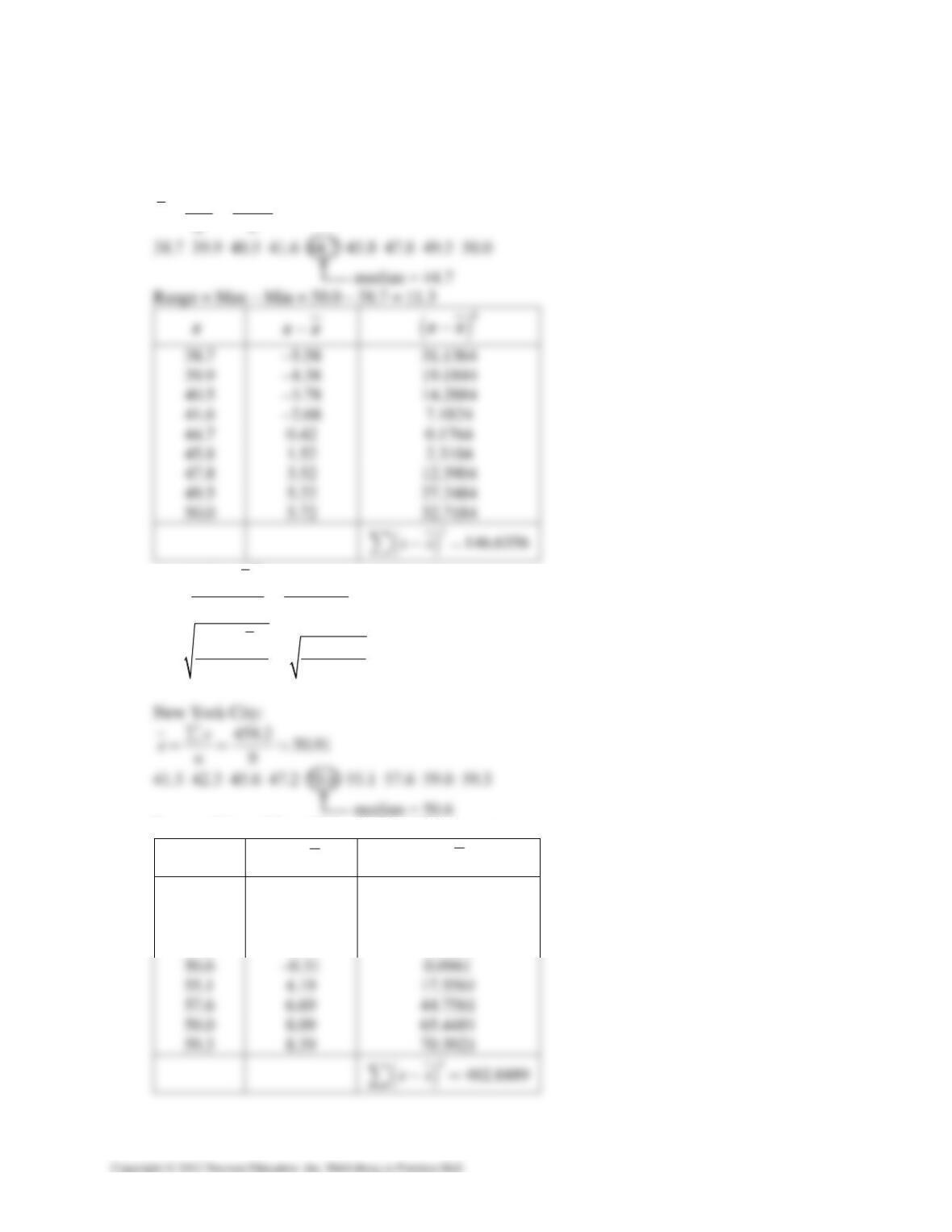
25a. Dallas:
398.5 44.28
x
x
x
xn
∑
== ≈
()
2
2146.6356 18.33
18
xx
sn
∑−
==≈
−
()
2
146.6356 4.28
18
xx
sn
∑−
==≈
−
Range = Max – Min = 59.3 – 41.5 = 17.8
x
−
x
x
()
−2
x
x
41.5 –9.41 88.5481
42.3 –8.61 74.1321
45.6 –5.31 28.1961
47.2 –3.71 13.7641
CHAPTER 2 │ DESCRIPTIVE STATISTICS 63
()
2
2402.8889 50.36
191
xx
sn
∑−
==≈
−−
()
2
402.8889 7.10
18
xx
sn
∑−
==≈
−
26a. Boston:
667.4 74.16
9
x
xn
∑
== ≈
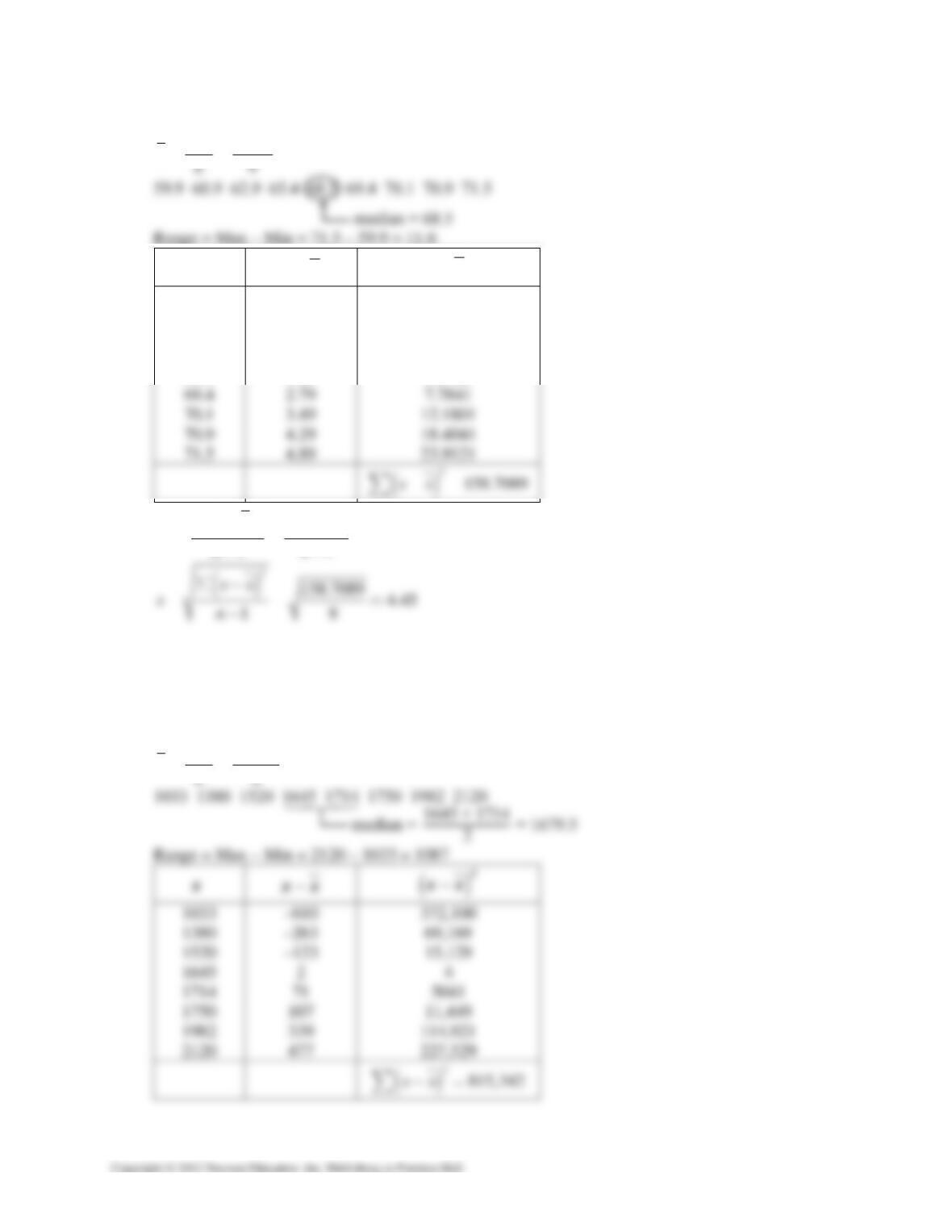
Range = Max – Min = 88.3 – 58.5 = 29.8
x
−
x
x
()
−2
x
x
58.5 –15.66 245.2356
64.5 –9.66 93.3156
69.9 –4.26 18.1476
()
2
2746.3624 93.30
191
xx
sn
∑−
==≈
−−
64 CHAPTER 2 │ DESCRIPTIVE STATISTICS
Chicago:
599.5 66.61
x
xn
∑
== ≈
x
−
x
x
()
−2
x
x
59.9 –6.71 45.0241
60.9 –5.71 32.6041
62.9 –3.71 13.7641
65.4 –1.21 1.4641
68.5 1.89 3.5721
()
2
2158.7089 19.84
xx
sn
∑−
==≈
b. It appears from the data that the annual salaries in Boston are more variable than the annual
salaries in Chicago. The annual salaries in Boston have higher mean and median than the
annual salaries in Chicago.
27a. Male:
13,144 1643
x
x
x
x
xn
∑
== =
CHAPTER 2 │ DESCRIPTIVE STATISTICS 65
()
2
2815,342 116, 477.4
181
xx
sn
∑−
==≈
−−
Female:
13,673 1709.1
8
x
xn
∑
== ≈
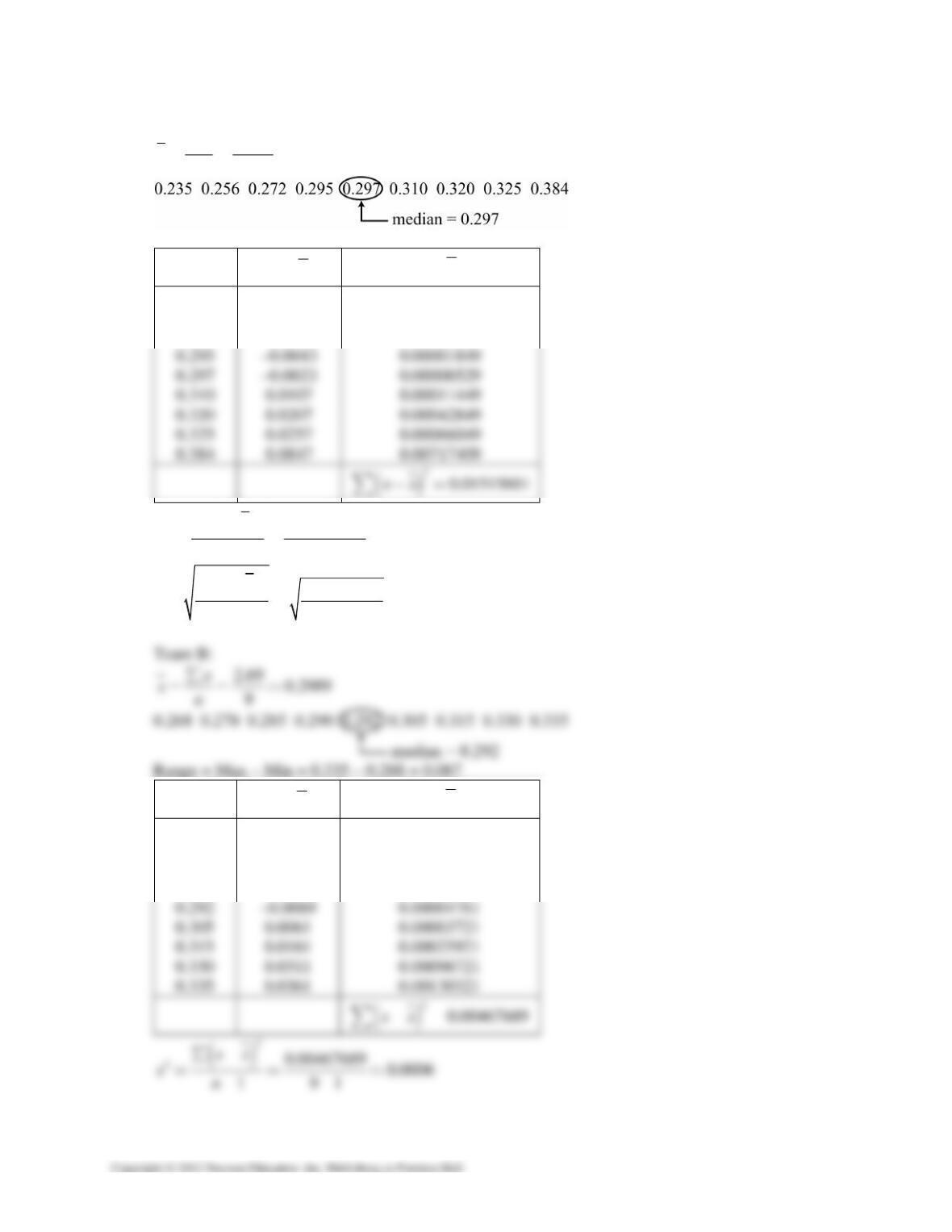
Range = Max – Min = 2210 – 1263 = 947
x
−
x
x
()
−2
x
x
1263 –446.1 199,005.21
1497 –212.1 44,986.41
()
2
2641,374.88 91,625.0
181
xx
sn
∑−
== ≈
−−
()
2
641,374.88 302.7
17
xx
sn
∑−
== =
−
66 CHAPTER 2 │ DESCRIPTIVE STATISTICS
28a. Team A:
2.694 0.2993
9
x
xn
∑
== ≈
Range = Max – Min = 0.384 – 0.235 = 0.149
x
−
x
x
()
−2
x
x
0.235 –0.0643 0.00413449
0.256 –0.0433 0.00187489
0.272 –0.0273 0.00074529
()
2
20.01515601 0.0019
191
xx
sn
∑−
== ≈
−−
()
2
0.01515601 0.0435
18
xx
sn
∑−
== =
−
x
−
x
x
()
−2
x
x
0.268 –0.0309 0.00095481
0.270 –0.0289 0.00083521
0.285 –0.0139 0.00019321
0.290 –0.0089 0.00007921
CHAPTER 2 │ DESCRIPTIVE STATISTICS 67
()
2
0.00467689 0.02418
18
xx
sn
∑−
== ≈
−
b. It appears form the data that the batting averages for Team A are more variable than the batting
averages for Team B. The batting averages for Team A have a higher mean and a higher
median than those for Team B.
30a. Greatest sample standard deviation: (i)
Data set (i) has more entries that are farther away from the mean.
Least sample standard deviation: (iii)
Data set (iii) has more entries that are close to the mean.
b. The three data sets have the same mean, median, and mode, but have different standard
deviations.
32a. Greatest sample standard deviation: (iii)
Data set (iii) has more entries that are farther away from the mean.
Least sample standard deviation: (i)
Data set (i) has more entries that are close to the mean.
b. The three data sets have the same mean and median but have different modes and standard
deviations.
35a. 75n=
68%(75) = (0.68)(75) 51 farms have values between $1300 and $1700 per acre.
b. 25n=
68%(25) = (0.68)(25) 17 farms have values between $1300 and $1700 per acre.
68 CHAPTER 2 │ DESCRIPTIVE STATISTICS
36a. 40n=
95%(40) = (0.95)(40) 38 farms have values between $1500 and $3300 per acre.
b. 20n=
95%(20) = (0.95)(20) 19 farms have values between $1500 and $3300 per acre.
38. 2400x= 450s=
{$1045, $1490, $3325, $3800} are outliers. They are more than 2 standard deviations from the
mean (1500, 3300). $1045 and $3800 are very unusual because they are more than 3 standard
deviations from the mean.
40.
()
2
2
111
11 10.75
4
2
k
−=− =−=
At least 75% of the 400-meter dash times lie within 2 standard deviations of the mean.
()
()
2 , 2 54.97, 59.17xsxs−+→
At least 75% of the 400-meter dash times lie between 54.97 and 59.17 seconds.
CHAPTER 2 │ DESCRIPTIVE STATISTICS 69
42.
43. Max Min 14 1 13
Class width = 2.6 3
555
−−
===⇒
Class Midpoint, x f xf
1-3 2 3 6
4-6 5 6 30
7-9 8 13 104
10-12 11 7 77
13-15 14 3 42
32N= 259xf =
∑
259 8.1
xf
µ∑
==≈
44. Max Min 244 145 99
Class width = 19.8 20
555
−−
===⇒
Class Midpoint, x f xf
145-164 154.5 8 1236.0
165-184 174.5 7 1221.5
70 CHAPTER 2 │ DESCRIPTIVE STATISTICS
3490 174.5
20
xf
N
µ∑
===
−xµ
()
−2
xµ
()
−2
x
fµ
–20 400 3200
0 0 0
45.
Midpoint, x f xf
70.5 1 70.5
92.5 12 1110.0
5725 114.5
50
xf
xn
∑
===
−
x
x
()
−2
x
x
()
−2
x
xf
–44 1936 1936
–22 484 5808
46.
x f xf
0 1 0
1 9 9
2 13 26
CHAPTER 2 │ DESCRIPTIVE STATISTICS 71
−
x
x
()
−2
x
x
()
−2
x
xf
–1.9 3.61 3.61
–0.9 0.81 7.29
129
−
47.
Class Midpoint, x f xf
0-4 2.0 22.1 44.20
5-14 9.5 43.4 412.30
15-19 17.0 21.2 360.40
12,100.15 37.17
325.5
xf
xn
∑
== ≈
−
x
x
()
−2
x
x
()
−2
x
xf
–35.17 1236.9289 27,336.12869
–27.67 765.6289 33,228.29426
–20.17 406.8289 8624.77268
–15.17 230.1289 5131.87447
72 CHAPTER 2 │ DESCRIPTIVE STATISTICS
48.
Midpoint, x f xf
4.5 35.4 159.30
14.5 35.3 511.85
24.5 33.5 820.75
34.5 33.6 1159.20
44.5 28.8 1281.60
6807.25 32.03
212.5
xf
xn
∑
== ≈
−
x
x
()
−2
x
x
()
−2
x
xf
–27.53 757.9009 26,829.69186
–17.53 307.3009 10,847.72117
–7.53 56.7009 1899.48015
2.47 6.1009 204.99024
12.47 155.5009 4478.42592
()
2
91, 287.88065 20.78
1 211.5
xxf
sn
∑−
== ≈
−
49. Summary Statistics:
Column n Mean Variance
Amount (in dollars) 15 58.8 239.74286
Std. Dev. Median Range Min Max
15.483632 60 59 30 89
CHAPTER 2 │ DESCRIPTIVE STATISTICS 73
51. Heights:
873 72.75
12
x
N
µ∑
===
x
−xµ
()
−2
xµ
68 –4.75 22.5625
69 –3.75 14.0625
69 –3.75 14.0625
70 –2.75 7.5625
()
2130.25 3.29
12
x
N
µ
σ∑−
==≈
heights
3.29
CV 100% 100 4.5%
72.75
σ
µ
=⋅ = ⋅ ≈
x
−xµ
()
−2
xµ
162 –25.83 667.1889
168 –19.83 393.2289
171 –16.83 283.2489
174 –13.83 191.2689
180 –7.83 61.3089
185 –2.83 8.0089
74 CHAPTER 2 │ DESCRIPTIVE STATISTICS
52a. Male:
x
2
x
1520 2,310,400
1750 3,062,500
2120 4,494,400
() ()
22
213,144
22,410,934 815,342
8341.3
1817
x
xn
sn
∑
∑− −
== =≈
−−
Female:
x
2
x
1785 3,186,225
1507 2,271,049
1497 2,241,009
∑ 224,010,241x=
∑
() ()
22
213,673
24,010,241 641,374.875
8302.7
181 7
x
xn
sn
∑
∑− −
== =≈
−−
b. The answers are the same as from Exercise 27.
53a. 41.5x≈ 5.3s≈
b. 43.6x≈ 5.6s≈
54a. 41.7x≈ 6.0s≈
b. 42.7x≈ 6.0s≈