2.7 Roots of Polynomials
1. Use synthetic division to deflate the given polynomial by the indicated root.
(a) p(x) = x4−2.25x3−25.75x2+ 28.5x+ 126, x∗= 3
(b) p(x) = x4+ 1.83x3−0.081x2+ 1.83x−1.081, x∗=−2.3
(c) p(x) = x4+ 20.5x3+ 129.5x2+ 230x−150, x∗= 0.5
(a) Let p(x) = x4−2.25x3−25.75x2+ 28.5x+ 126. Applying synthetic division
to pwith x∗= 3 yields
(b) Let p(x) = x4+1.83x3−0.081x2+1.83x−1.081. Applying synthetic division
(c) Let p(x) = x4+ 20.5x3+ 129.5x2+ 230x−150. Applying synthetic division
2. Apply Laguerre’s method to each of the following polynomials with a starting
approximation of x0= 0 and a convergence tolerance of 5 ×10⁻¹¹.
(a) p(x) = x3−4x2−3x+ 5
(b) p(x) = x3−7x2+ 14x−6
(c) p(x) = x4+ 20.5x3+ 129.5x2+ 230x−150
(d) p(x) = x4−2x3−5x2+ 12x−5
(a) Let p(x) = x3−4x2−3x+ 5 and take x0= 0 as an initial approximation and
With these values we now calculate
therefore,
These values then lead to
Roots of Polynomials 3
From here, we calculate
From here, we calculate
With these values we now calculate
Since Gis negative, we choose the negative sign in front of the radical in the
4Section 2.7
These values then lead to
Once again, |a|> ǫ, so we perform a third iteration. Evaluating p,p′and p′′
From here, we calculate
(c) Let p(x) = x4+ 20.5x3+ 129.5x2+ 230x−150 and take x0= 0 as an initial
With these values we now calculate
Roots of Polynomials 5
therefore,
These values then lead to
Once again, |a|> ǫ, so we perform a third iteration. Evaluating p,p′and p′′
From here, we calculate
(d) Let p(x) = x4−2x3−5x2+12x−5and take x0= 0 as an initial approximation
6Section 2.7
therefore,
These values then lead to
From here, we calculate
Roots of Polynomials 7
3. Construct an algorithm to deflate the n-th degree polynomial
p(x) = anxn+an−1xn−1+an−2xn−2+···+a1x+a0
by the quadratic factor x2+αx +β;i.e., find the polynomial
q(x) = bn−2xn−2+bn−3xn−3+bn−4xn−4+···+b1x+b0
such that p(x) = (x2+αx +β)q(x).
Expand the product
4. Determine all roots for each of the following polynomials. Use a convergence
tolerance of 5 ×10⁻¹¹.
(a) p(x) = 2x5−6x4+ 5x3+x2+ 2
(b) p(x) = −3x6+x3+ 10x−1
(c) p(x) = x6+x5−9x4−8x3+ 29x2−4x+ 4
(d) p(x) = x4+ 5x3+ 7x2+ 1
(e) p(x) = 16x4−40x3+ 5x2+ 20x+ 6
(f) p(x) = 10x3−8.3x2+ 2.295x−0.21141
8Section 2.7
(b) Let p(x) = −3x6+x3+ 10x−1. The roots of pare:
(c) Let p(x) = x6+x5−9x4−8x3+ 29x2−4x+ 4. The roots of pare:
(d) Let p(x) = x4+ 5x3+ 7x2+ 1. The roots of pare:
(e) Let p(x) = 16x4−40x3+ 5x2+ 20x+ 6. The roots of pare:
5. The Chebyshev polynomials, Ti(x), are a special class of functions. They satisfy
the two-term recurrence relation
Ti+1(x) = 2xTi(x)−Ti−1(x)
with T0(x) = 1 and T1(x) = x.
(a) Using the recurrence relation, determine the formula for T6(x).
(b) Locate all roots of T6(x).
(a) With T0(x) = 1 and T1(x) = x, we calculate
6. The Hermite polynomials, Hi(x), are a special class of functions. They satisfy
the two-term recurrence relation
Hi+1(x) = 2xHi(x)−2iHi−1(x)
with H0(x) = 1 and H1(x) = x.
(a) Using the recurrence relation, determine the formula for H5(x).
(b) Locate all roots of H5(x).
(a) With H0(x) = 1 and H1(x) = 2x, we calculate
10 Section 2.7
7. The Laguerre polynomials, Li(x), are a special class of functions. They satisfy
the two-term recurrence relation
Li+1(x) = (1 + 2i−x)Li(x)−i2Li−1(x)
with L0(x) = 1 and L1(x) = 1 −x.
(a) Using the recurrence relation, determine the formula for L4(x).
(b) Locate all roots of L4(x).
(a) With L0(x) = 1 and L1= 1 −x, we calculate
8. The Legendre polynomials, Pi(x), are a special class of functions. They satisfy
the two-term recurrence relation
Pi+1(x) = 2i+ 1
i+ 1 xPi(x)−i
i+ 1Pi−1(x)
with P0(x) = 1 and P1(x) = x.
(a) Using the recurrence relation, determine the formula for P5(x).
(b) Locate all roots of P5(x).
Roots of Polynomials 11
9. The concentration, C, of a certain chemical in the bloodstream thours after
injection into muscle tissue is given by
C=3t2+t
50 + t3.
At what time is the concentration greatest?
Using Laguerre’s method with an initial approximation of x0= 0 and a conver-
10. DeSanti (“A Model for Predicting Aircraft Altitude Loss in a Pull-Up from
a Dive,” SIAM Review, 30 (4), pp. 625 – 628, 1988) develops the following
relationship for the ratio between the final velocity, Vf, and the initial velocity,
V0, for an aircraft executing a pull-up from a dive:
1
3Vf
V03
−BVf
V0
−1
3+Bcos γ0= 0.
γ0is the initial flight path angle and B=g/(kV 2
0), where gis the acceleration
due to gravity and kis related to the coefficient of lift. The altitude loss during
the pull-up can be determined from the ratio Vf/V0using the equation
∆y=1−(Vf/V0)2
2kB .
Determine the altitude loss associated with each of the following sets of system
parameters (take g= 9.8 m/s2):
(a) V0= 100 m/s, γ0=−30◦,k= 0.00196 m−1
(b) V0= 150 m/s, γ0=−10◦,k= 0.00145 m−1
(c) V0= 200 m/s, γ0=−45◦,k= 0.00128 m−1
(d) V0= 250 m/s, γ0=−30◦,k= 0.00112 m−1
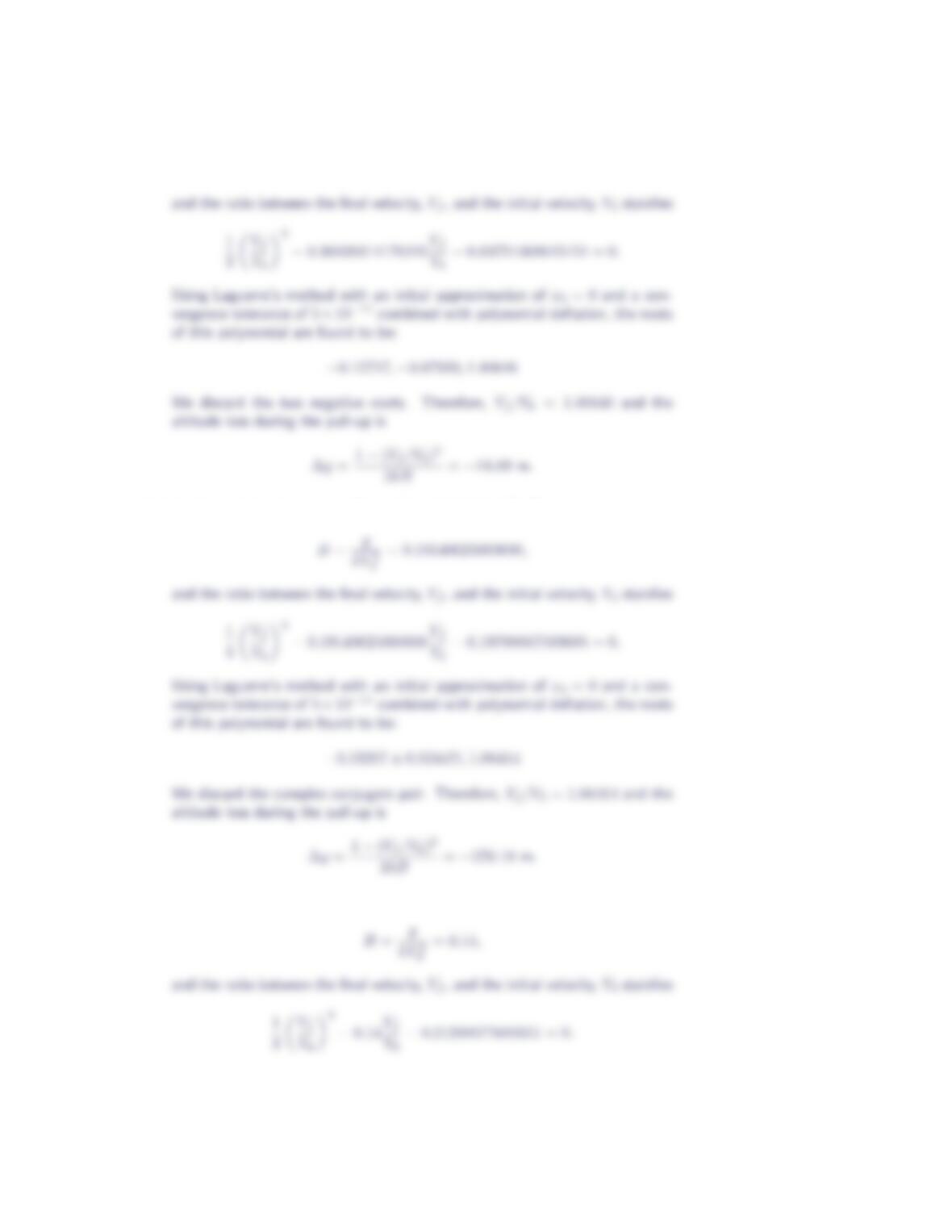
(a) Let V0= 100 m/s, γ0=−30◦and k= 0.00196 m−1. Then
Using Laguerre’s method with an initial approximation of x0= 0 and a con-
(b) Let V0= 150 m/s, γ0=−10◦and k= 0.00145 m−1. Then
Roots of Polynomials 13
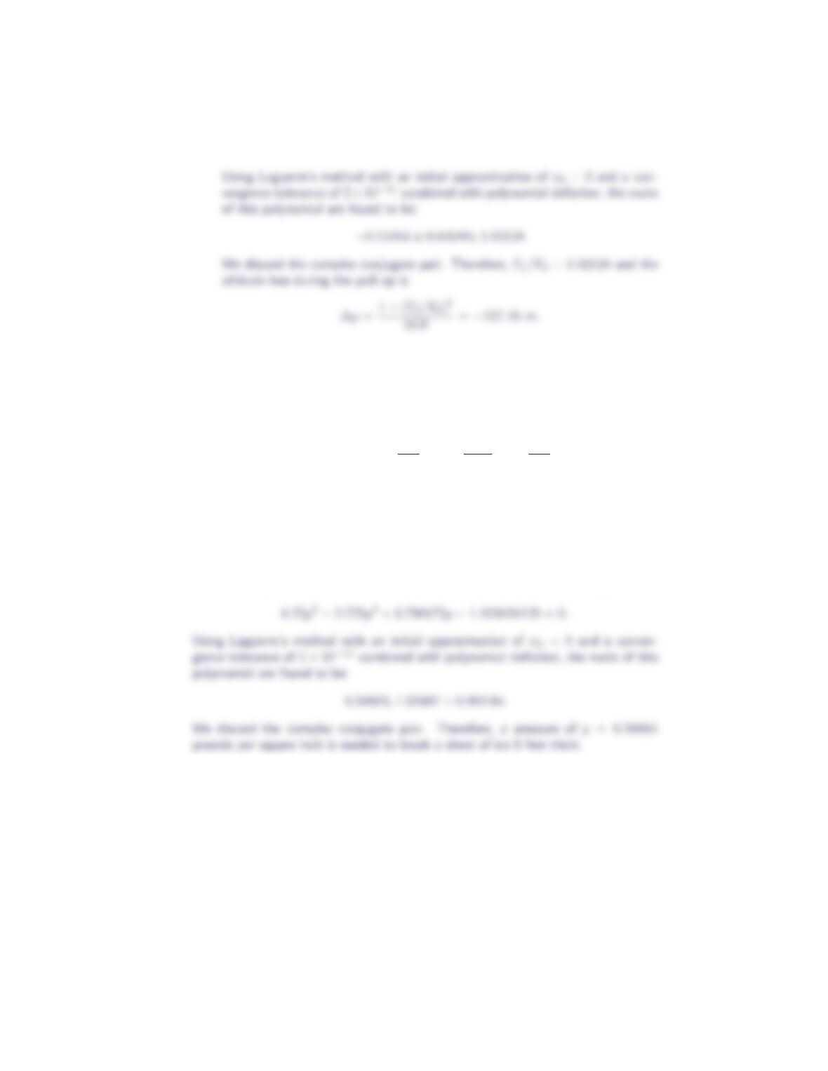
(c) Let V0= 200 m/s, γ0=−45◦and k= 0.00128 m−1. Then
(d) Let V0= 250 m/s, γ0=−30◦and k= 0.00112 m−1. Then
14 Section 2.7
11. In determining the minimum cushion pressure needed to break a given thickness
of ice using an air cushion vehicle, Muller (“Ice Breaking with an Air Cushion
Vehicle,” in Mathematical Modeling: Classroom Notes in Applied Mathematics,
M.S. Klamkin, editor, SIAM, 1987) derived the equation
p3(1 −β2) + 0.4hβ2−σh2
r2p2+σ2h4
3r4p−σh2
3r23
= 0,
where pdenotes the cushion pressure, hthe thickness of the ice field, rthe size
of the air cushion, σthe tensile strength of the ice, and βis related to the width
of the ice wedge. Taking β= 0.5, r= 40 feet and σ= 150 pounds per square
inch (psi), determine the cushion pressure needed to break a sheet of ice 6 feet
thick.
Substituting β= 0.5,r= 40,σ= 150 and h= 6 into the equation for pyields
12. Determine the roots of the polynomials
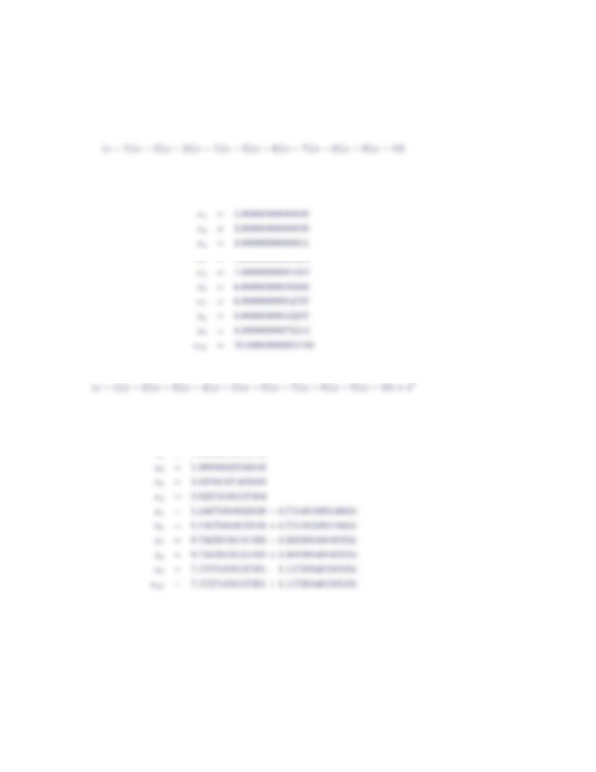
P(x) = (x−1)(x−2)(x−3)(x−4)(x−5)(x−6)(x−7)(x−8)(x−9)(x−10)
and
˜
P(x) = (x−1)(x−2)(x−3)(x−4)(x−5)(x−6)(x−7)(x−8)(x−9)(x−10)+x5
with Laguerre’s method as the central rootfinding scheme. Apply a convergence
tolerance of 5 ×10⁻¹¹, and take 0 as the initial approximation.
Roots of Polynomials 15
Expanding the polynomial
and then using Laguerre’s method with an initial approximation of x0= 0 and a
convergence tolerance of 5×10⁻¹¹ combined with polynomial deflation, the roots
of this polynomial are found to be:
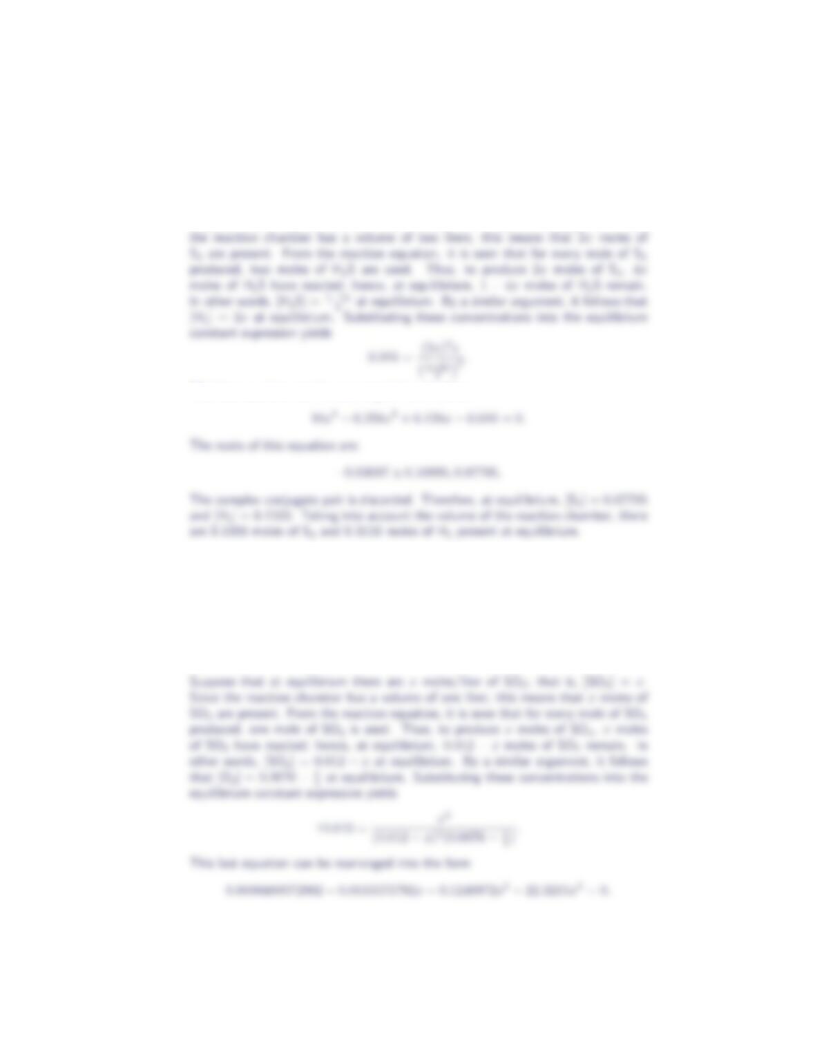
On the other hand, expanding the polynomial
and then using Laguerre’s method with an initial approximation of x0= 0 and a
convergence tolerance of 5×10⁻¹¹ combined with polynomial deflation, the roots
of this polynomial are found to be:
x1= 1.00000275579138
13. One mole of H2S is injected into a two liter reaction chamber, and the reversible
reaction
2H2S⇀
↽2H2+ S2
16 Section 2.7
is allowed to proceed to equilibrium. If the equilibrium constant for the indicated
reaction is k= 0.016, how much H2and S2are present at equilibrium?
Suppose that at equilibrium there are xmoles/liter of S2; that is, [S2] = x. Since
This last equation can be rearranged into the form
14. The reversible reaction
2SO2+ O2⇀
↽2SO3
is allowed to proceed to equilibrium in a one liter reaction chamber. If 0.012
moles of SO2and 0.0076 moles of O2are initially present and the equilibrium
constant for the indicated reaction is k= 44.643, how much SO3is present at
equilibrium?
Roots of Polynomials 17
The roots of this equation are: