Case 2-25 (30 minutes)
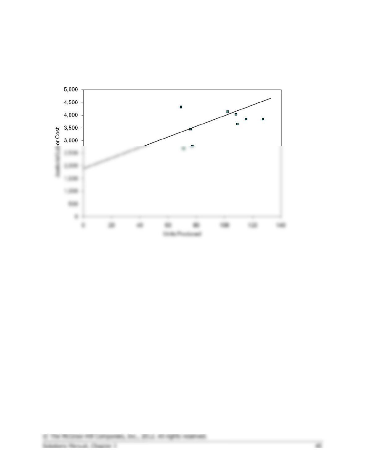
1. The scattergraph of janitorial labor cost versus the number of units
produced is presented below:
Case 2-25 (continued)
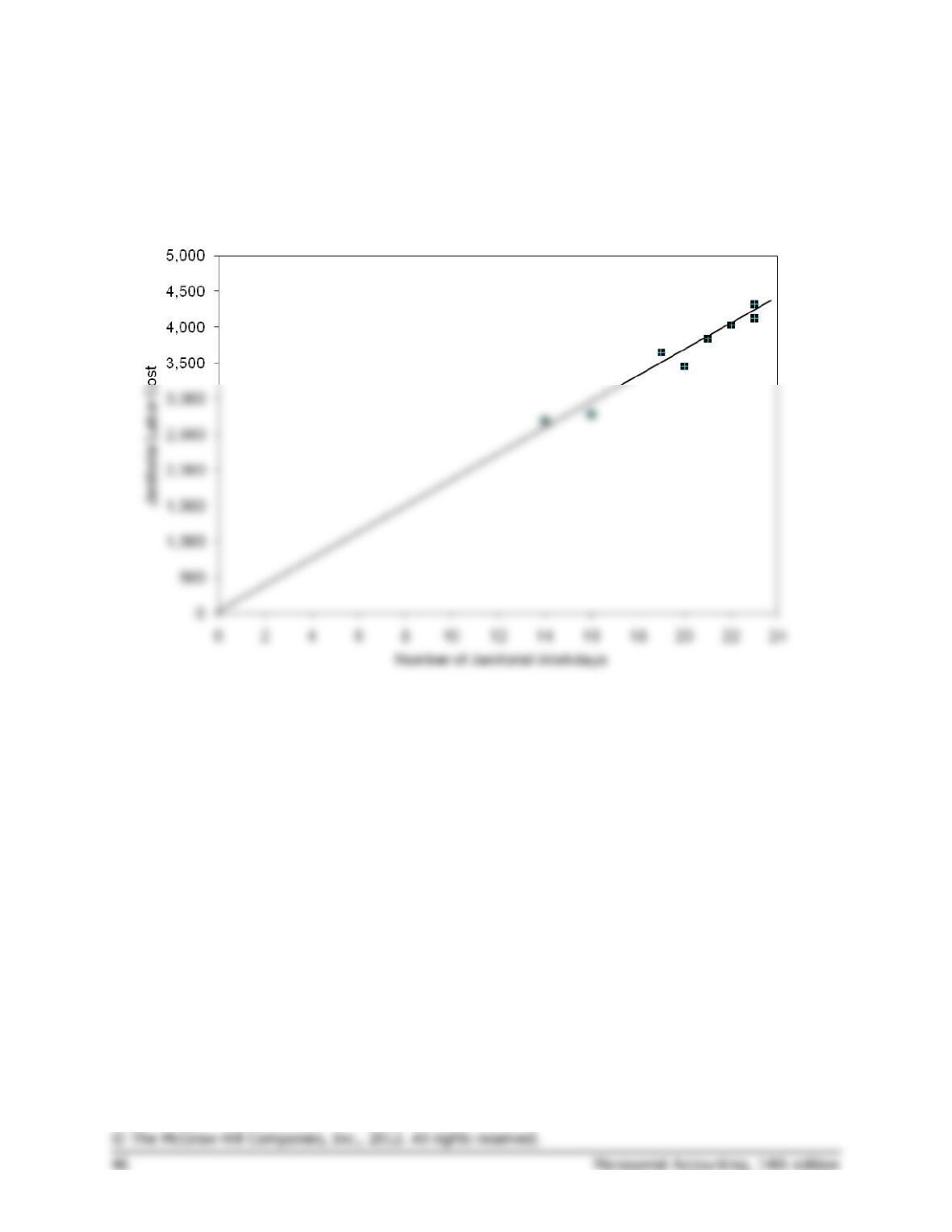
2. The scattergraph of the janitorial labor cost versus the number of
janitorial workdays is presented below:
Case 2-25 (continued)
3. The number of workdays should be used as the activity base rather than
the number of units produced. There are several reasons for this. First,
the scattergraphs reveal that there is a much stronger relationship (i.e.,
higher correlation) between janitorial costs and number of workdays
than between janitorial costs and number of units produced. Second,
Case 2-26 (60 minutes)
1. High-low method:
Hours
Cost
High level of activity ……..
25,000
$99,000
Low level of activity ……..
10,000
Change ……………………..
15,000
$34,500
Fixed element …………………………………
$41,500
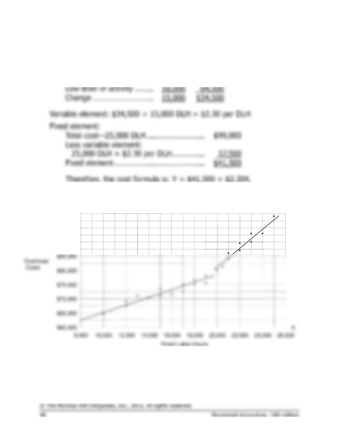
2. The scattergraph is shown below:
$60,000
$65,000
$70,000
$75,000
$80,000
$85,000
10,000
12,000
14,000
16,000
18,000
20,000
22,000
24,000
26,000
$90,000
$95,000
$100,000
Y
Case 2-26 (continued)
2. The scattergraph shows that there are two relevant ranges—one below
19,500 DLH and one above 19,500 DLH. The change in equipment lease
3. The cost formulas computed with the high-low and regression methods
are faulty since they are based on the assumption that a single straight
line provides the best fit to the data. Creating two data sets related to
the two relevant ranges will enable more accurate cost estimates.
4. High-low method:
Hours
Cost
High level of activity ……..
25,000
$99,000
Low level of activity ……..
20,000
80,000
Change ……………………..
5,000
$19,000
Total cost—25,000 DLH …………………….
$99,000
Fixed element …………………………………
Variable cost: 22,500 hours × $3.80 per hour ………..
Fixed cost ………………………………………………………
4,000
Total cost ……………………………………………………….
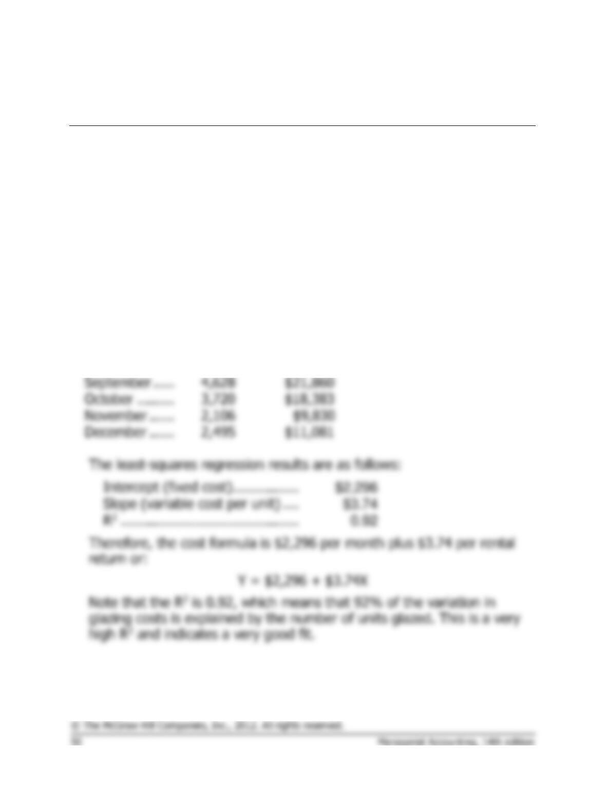
5. The high-low estimate of fixed costs is $6,090 lower than the estimate
provided by least-squares regression. The high-low estimate of the
variable cost per machine hour is $0.27 higher than the estimate
Appendix 2A
Least-Squares Regression Computations
Exercise 2A–1 (20 minutes)
1.
Month
Rental
Returns
(X)
Car Wash Costs
(Y)
January ……….
2,310
$10,113
February ……..
2,453
$12,691
March …………
2,641
$10,905
April……………
2,874
$12,949
May ……………
3,540
$15,334
June …………..
4,861
$21,455
July ……………
5,432
$21,270
August ………..
5,268
$19,930
September …..
4,628
$21,860
October ………
3,720
$18,383
November ……
2,106
December ……
2,495
$11,081
Intercept (fixed cost) …………….
Slope (variable cost per unit) ….

Exercise 2A–1 (continued)
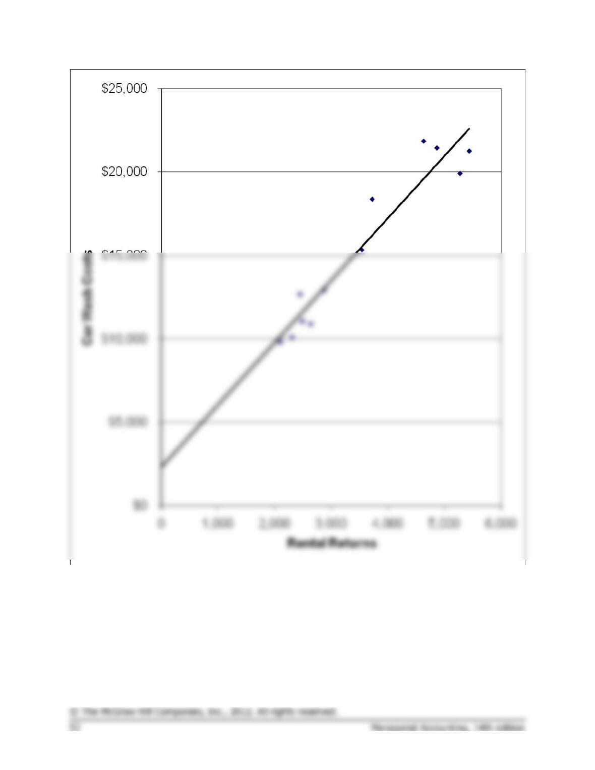
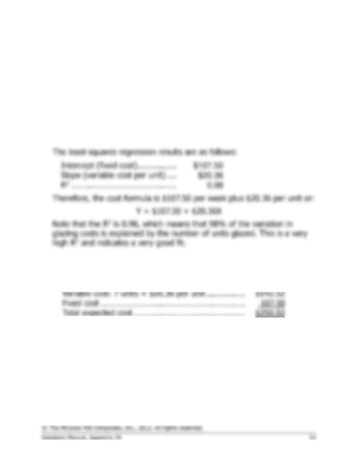
While not a requirement of the exercise, it is always a good to plot the data
on a scattergraph. The scattergraph can help spot nonlinearities or other
problems with the data. In this case, the regression line (shown below) is a
reasonably good approximation to the relationship between car wash costs
and rental returns.
Exercise 2A-2 (30 minutes)
1.
Week
Units
(X)
Total Glazing Cost
(Y)
1
8
$270
2
5
$200
3
10
$310
4
4
$190
5
6
$240
6
9
$290
Intercept (fixed cost) …………….
Slope (variable cost per unit) ….
2. Y = $107.50 + $20.36X
3. Total expected glazing cost if 7 units are processed:
Variable cost: 7 units × $20.36 per unit …………….
Fixed cost …………………………………………………..
Total expected cost ……………………………………….
Problem 2A-3 (45 minutes)
1.
Number of Leagues
(X)
Total Cost
(Y)
5
$13,000
2
$7,000
4
$10,500
6
$14,000
3
$10,000
Intercept (fixed cost) ……………….
$4,100
Slope (variable cost per unit) …….
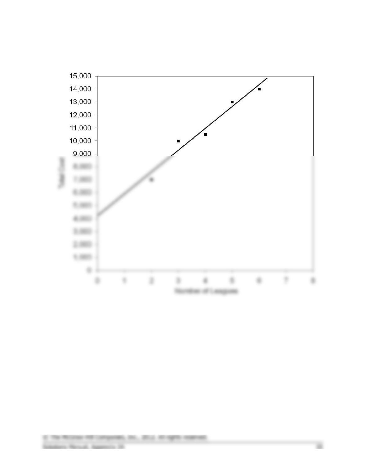
2. Y = $4,100 + $1,700X
3. The expected total cost for 7 leagues would be:
Fixed cost …………………………………………………
$ 4,100
Variable cost (7 leagues × $1,700 per league) …..
11,900
Total cost ………………………………………………….
$16,000
Problem 2A-3 (continued)
4.
Problem 2A-4 (45 minutes)
1. a.
Quarter
Tons
Mined
(X)
Utilities
Cost
(Y)
Year 1:
1st
15,000
$50,000
2nd
11,000
$45,000
21,000
$60,000
12,000
$75,000
Year 2:
1st
18,000
25,000
30,000
$85,000
28,000
The least-squares regression results are as follows:
Intercept (fixed cost) …………….
$28,352
Slope (variable cost per unit) ….
$2.58
R2 …………………………………….
0.47
Problem 2A-4 (continued)
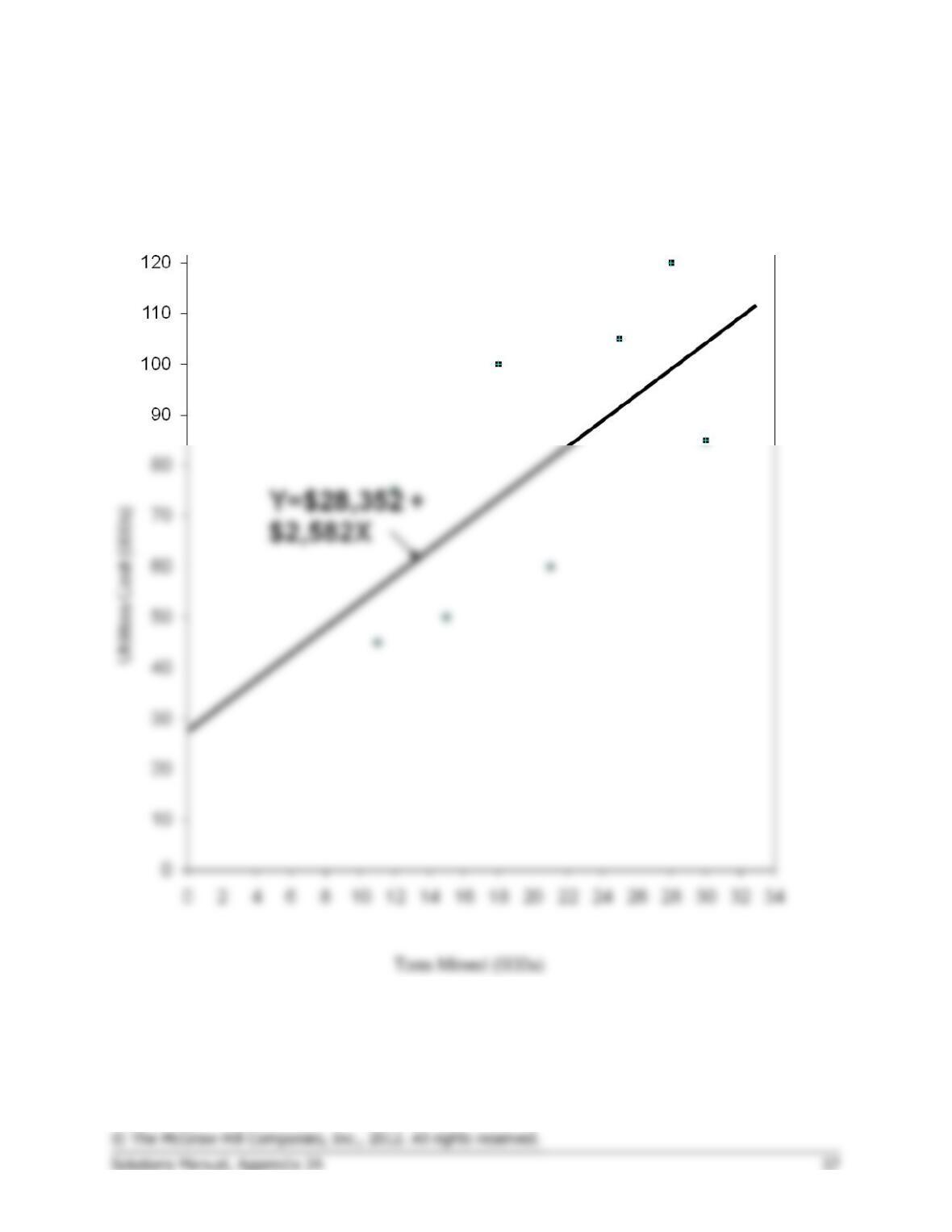
b. The scattergraph plot of utility costs versus tons mined appears
below: