PROBLEM 2.1
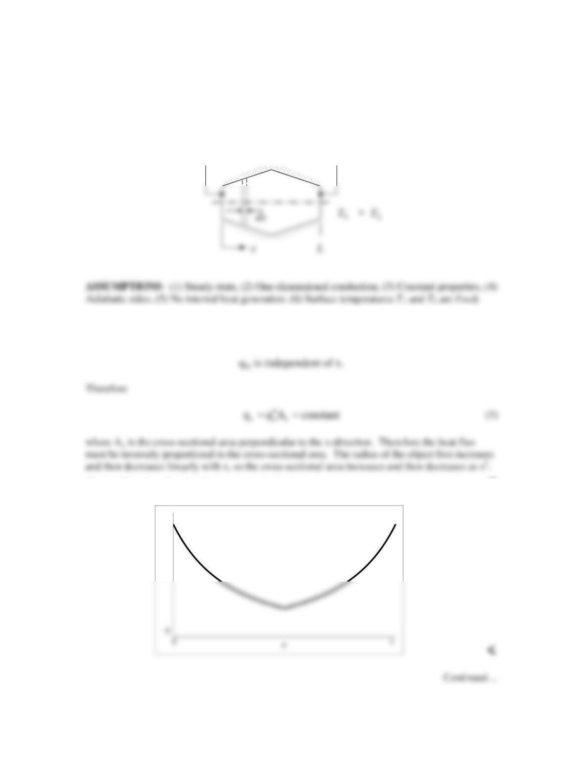
KNOWN: Axisymmetric object with varying cross–sectional area and different temperatures at
its two ends, insulated on its sides.
FIND: Shapes of heat flux distribution and temperature distribution.
SCHEMATIC:
ANALYSIS: For the prescribed conditions, it follows from conservation of energy, Eq. 1.12c,
that for a differential control volume,
.E E or q q
in out x x+dx
= =
Hence
The resulting heat flux distribution is sketched below. <
q”
T2
T1
PROBLEM 2.1 (Cont.)
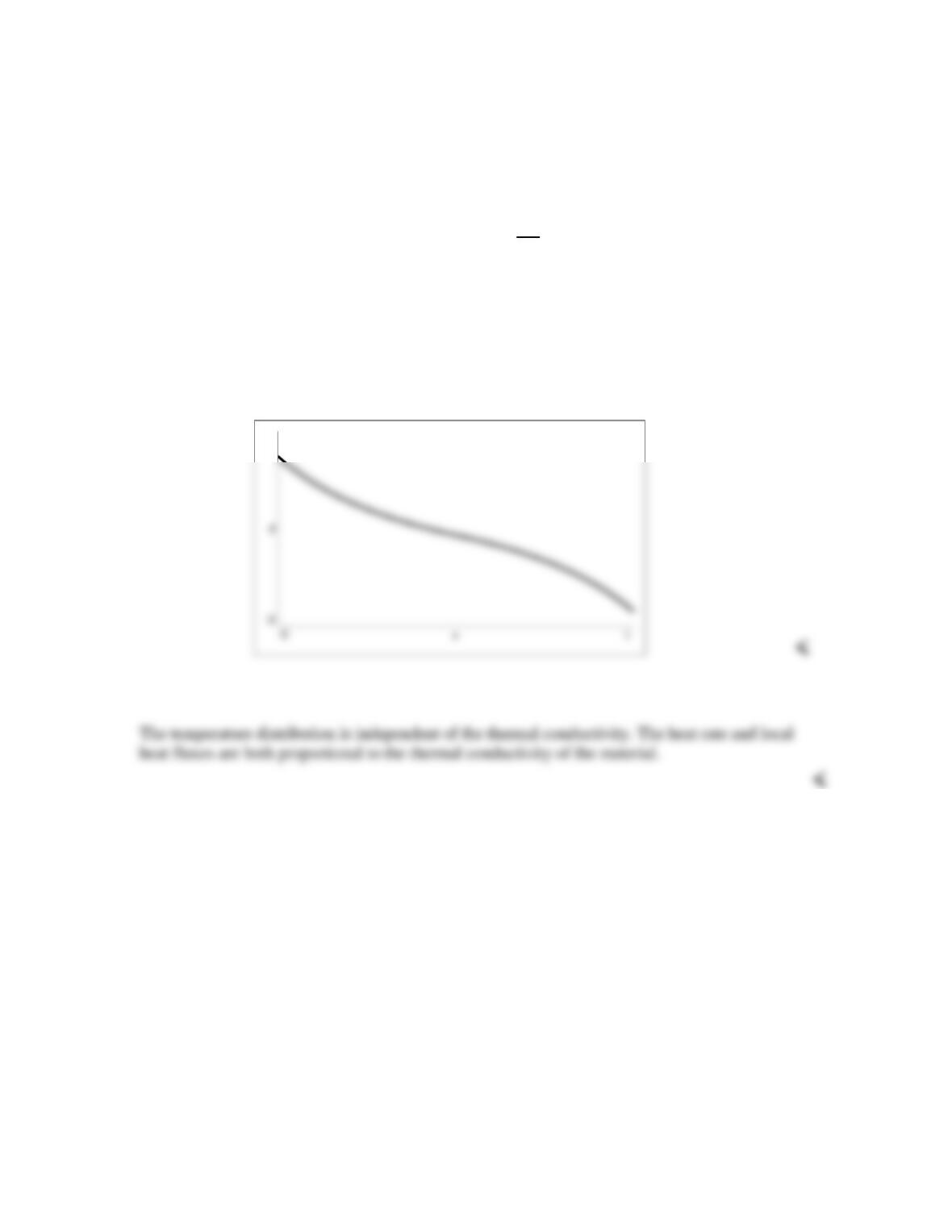
To find the temperature distribution, we can use Fourier’s law:
x
dT
qk
dx
′′ = −
(2)
Therefore the temperature gradient is negative and its magnitude is proportional to the heat flux.
The temperature decreases most rapidly where the heat flux is largest and more slowly where the
heat flux is smaller.
Based on the heat flux plot above we can prepare the sketch of the temperature distribution
below.
COMMENTS: If the heat rate was fixed the temperature difference, T1 – T2, would be
inversely proportional to the thermal conductivity. The temperature distribution would be of the
same shape, but local temperatures T(x) would vary as the thermal conductivity is adjusted.
PROBLEM 2.2
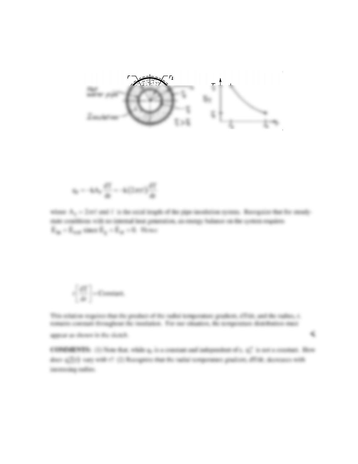
KNOWN: Hot water pipe covered with thick layer of insulation.
FIND: Sketch temperature distribution and give brief explanation to justify shape.
SCHEMATIC:
ASSUMPTIONS: (1) Steady-state conditions, (2) One-dimensional (radial) conduction, (3) No
internal heat generation, (4) Insulation has uniform properties independent of temperature and
position.
ANALYSIS: Fourier’s law, Eq. 2.1, for this one-dimensional (cylindrical) radial system has the form
qr = Constant.
That is, qr is independent of radius (r). Since the thermal conductivity is also constant, it follows that
PROBLEM 2.3
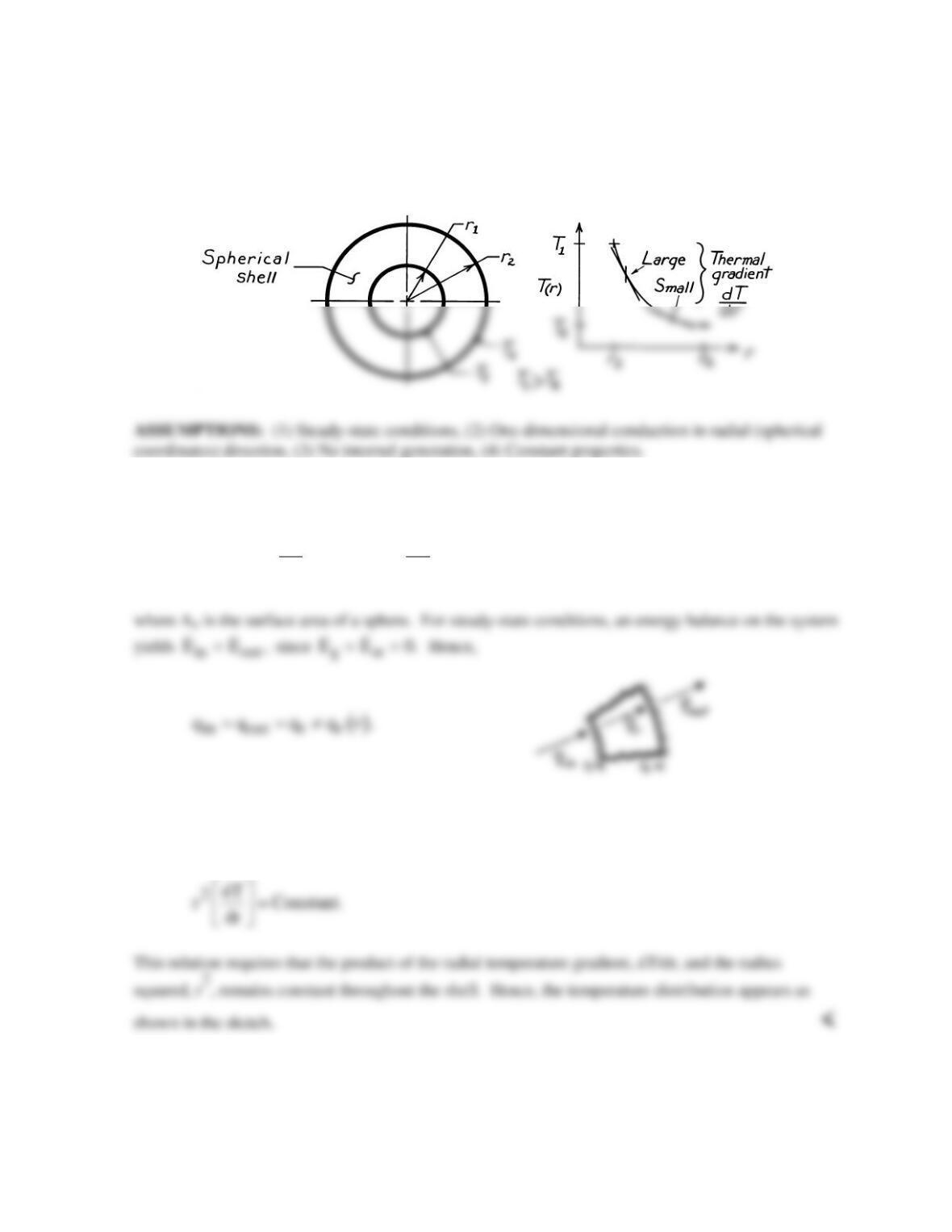
KNOWN: A spherical shell with prescribed geometry and surface temperatures.
FIND: Sketch temperature distribution and explain shape of the curve.
SCHEMATIC:
ANALYSIS: Fourier’s law, Eq. 2.1, for this one-dimensional, radial (spherical coordinate) system
has the form
()
2
rr
dT dT
q k A k 4 r
dr dr
π
=−=−
That is, qr is a constant, independent of the radial coordinate. Since the thermal conductivity is
constant, it follows that
COMMENTS: Note that, for the above conditions,
( )
rr
q q r;≠
that is, qr is everywhere constant.
How does
′′
q
r
vary as a function of radius?
PROBLEM 2.4
KNOWN: Temperature dependence of the thermal conductivity, k(T), for heat transfer through a
plane wall.
FIND: Effect of k(T) on temperature distribution, T(x).
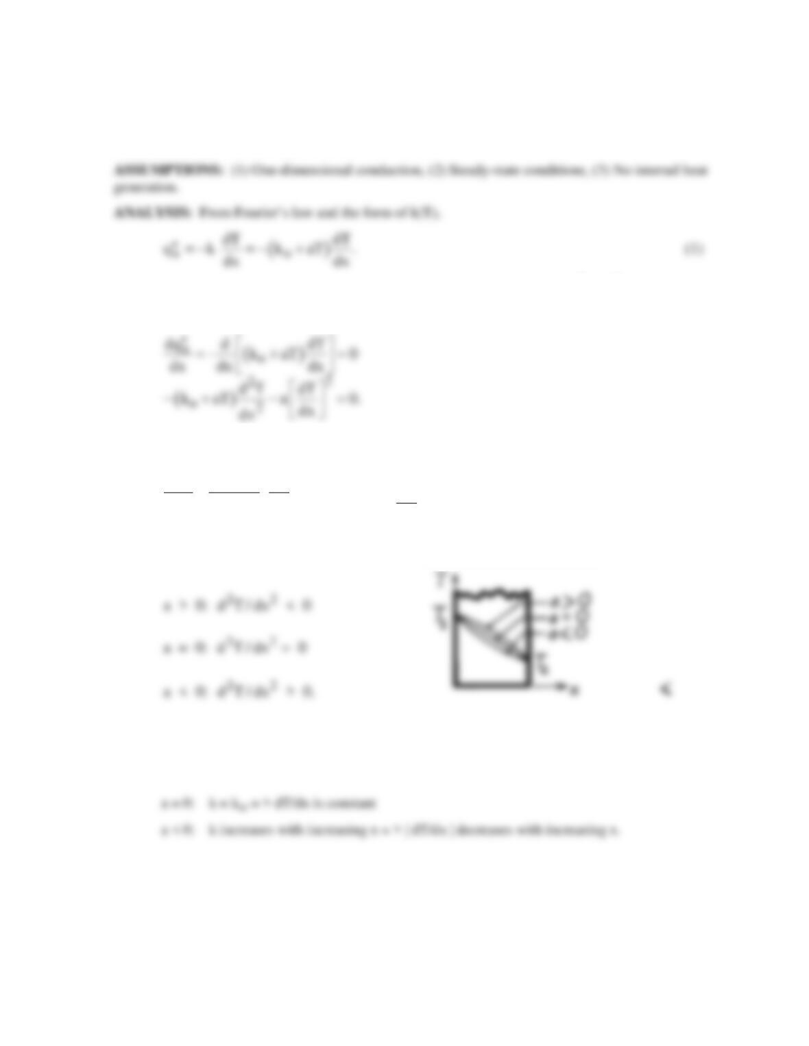
The shape of the temperature distribution may be inferred from knowledge of d2T/dx2 = d(dT/dx)/dx.
Since
′′
qx
is independent of x for the prescribed conditions,
Hence,
o
2
22
2o
k aT=k>0
d T -a dT where dT 0
k aT dx
dx dx
+
=
>
+
from which it follows that for
COMMENTS: The shape of the distribution could also be inferred from Eq. (1). Since T decreases
with increasing x,
a > 0: k decreases with increasing x = > | dT/dx | increases with increasing x
PROBLEM 2.5
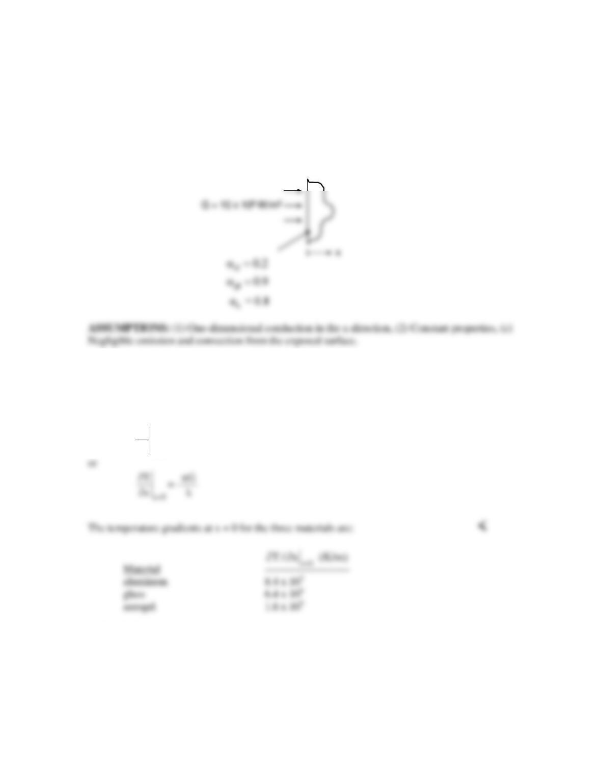
KNOWN: Irradiation and absorptivity of aluminum, glass and aerogel.
FIND: Ability of the protective barrier to withstand the irradiation in terms of the temperature
gradients that develop in response to the irradiation.
SCHEMATIC:
PROPERTIES: Table A.1, pure aluminum (300 K): kal = 238 W/m⋅K. Table A.3, glass (300 K):
kgl = 1.4 W/m⋅K.
ANALYSIS: From Eqs. 1.6 and 2.32
s abs
x=0
T
-k = q = G = αG
x
∂′′
∂
COMMENT: It is unlikely that the aerogel barrier can sustain the thermal stresses associated
with the large temperature gradient. Low thermal conductivity solids are prone to large
temperature gradients, and are often brittle.
PROBLEM 2.6
KNOWN: One–dimensional system with prescribed thermal conductivity and thickness.
FIND: Unknowns for various temperature conditions and sketch distribution.
SCHEMATIC:
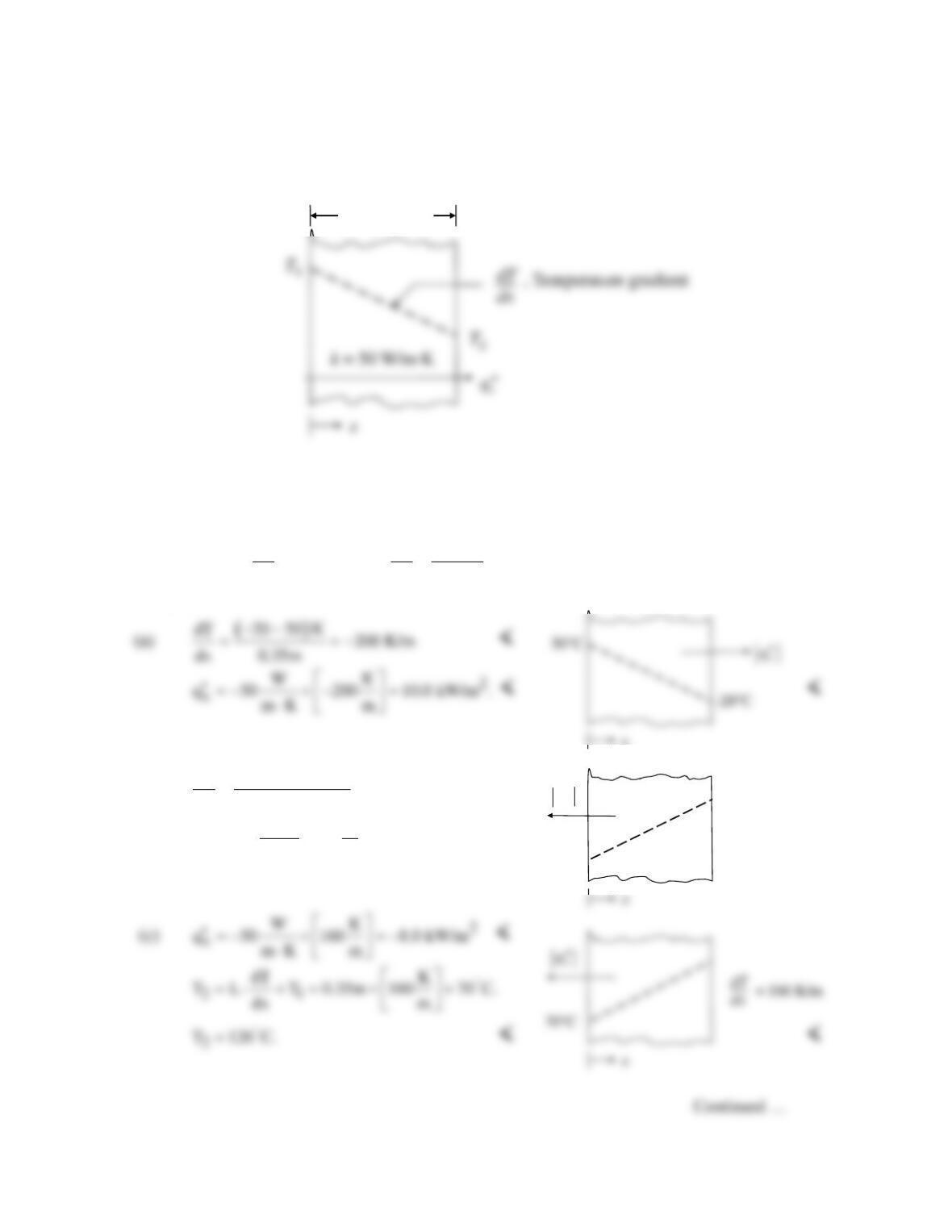
L= 0.35 m
ASSUMPTIONS: (1) Steady-state conditions, (2) One-dimensional conduction, (3) No internal heat
generation, (4) Constant properties.
ANALYSIS: The rate equation and temperature gradient for this system are
21
x
dT dT T T
q k and .
dx dx L
−
′′ =−=
(1,2)
Using Eqs. (1) and (2), the unknown quantities for each case can be determined.
(b)
( )
( )
10 30 K
dT 57 K/m
dx 0.35m
− −−
= =
<
2
x
WK
q 50 57 2.86 kW/m .
mK m
′′ =−×=−
⋅
< <
x
-10°C
-30°C
q
x
“
PROBLEM 2.6 (Cont.)
(d)
2
x
WK
q 50 80 4.0 kW/m
mK m
′′ =− ×− =
⋅
<
12
dT K
T T L 40 C 0.35m 80
dx m
= −⋅ = − −
<
40°C
qx
“
dT
dx = -80 K/m
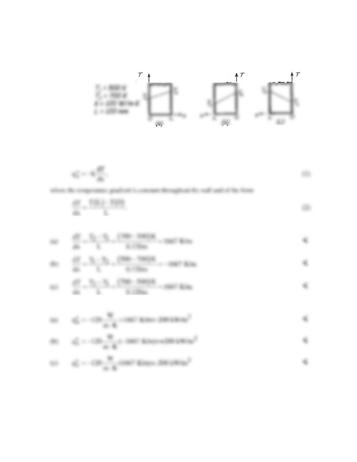
PROBLEM 2.7
KNOWN: Plane wall with prescribed thermal conductivity, thickness, and surface temperatures.
FIND: Heat flux,
′′
q
x
, and temperature gradient, dT/dx, for the three different coordinate systems
shown.
SCHEMATIC:
ASSUMPTIONS: (1) One-dimensional heat flow, (2) Steady-state conditions, (3) No internal
generation, (4) Constant properties.
ANALYSIS: The rate equation for conduction heat transfer is
Substituting numerical values, find the temperature gradients,
The heat rates, using Eq. (1) with k = 120 W/m⋅K, are
PROBLEM 2.8
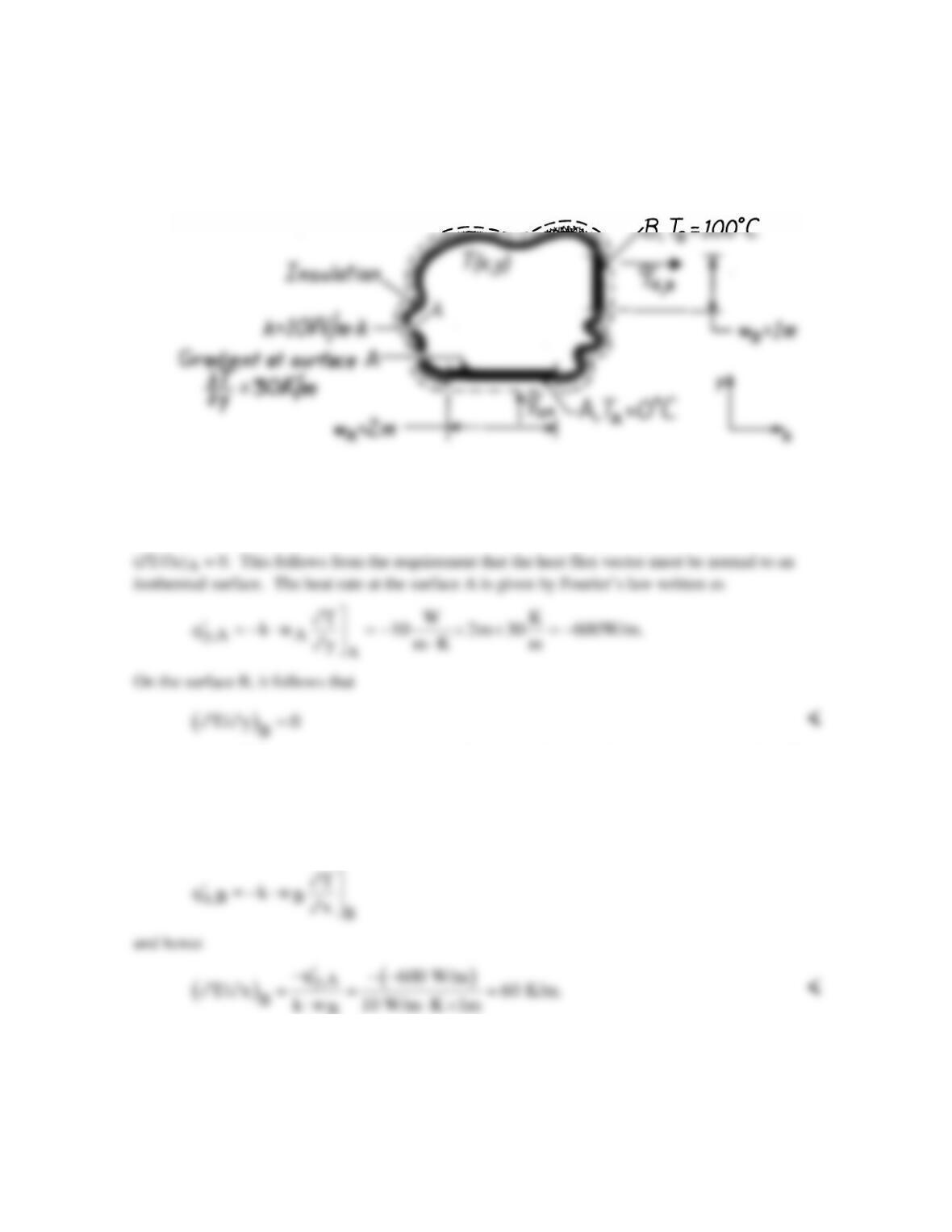
KNOWN: Two-dimensional body with specified thermal conductivity and two isothermal surfaces
of prescribed temperatures; one surface, A, has a prescribed temperature gradient.
FIND: Temperature gradients, ∂T/∂x and ∂T/∂y, at the surface B.
SCHEMATIC:
ASSUMPTIONS: (1) Two-dimensional conduction, (2) Steady-state conditions, (3) No heat
generation, (4) Constant properties.
ANALYSIS: At the surface A, the temperature gradient in the x-direction must be zero. That is,
in order to satisfy the requirement that the heat flux vector be normal to the isothermal surface B.
Using the conservation of energy requirement, Eq. 1.12c, on the body, find
′−′=′=′
q q or q q
y,Ax,Bx,By,A
0 .
Note that,
COMMENTS: Note that, in using the conservation requirement,
′= + ′
q q
in y,A
and
′= + ′
q q
out x,B.
PROBLEM 2.9
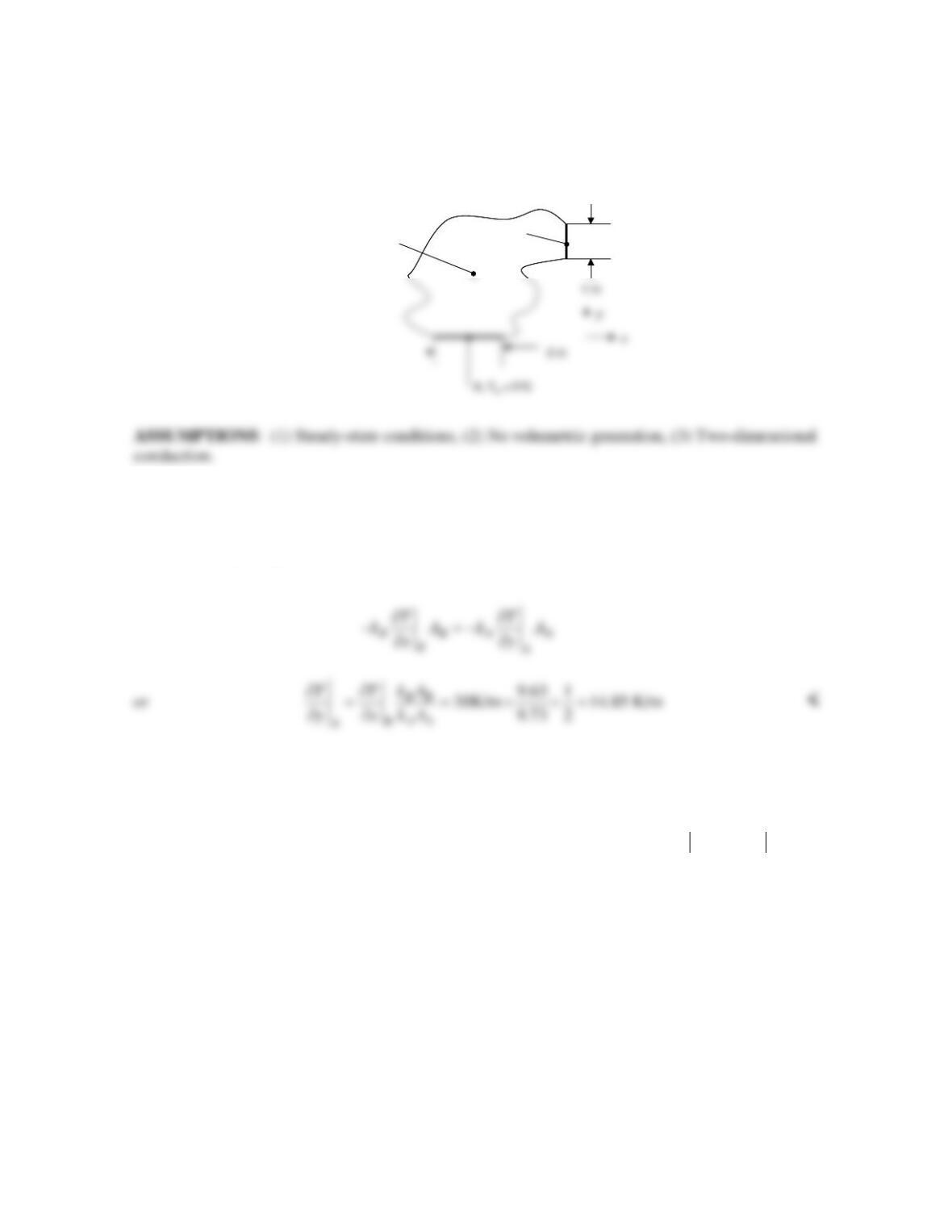
KNOWN: Temperature, size and orientation of Surfaces A and B in a two-dimensional geometry.
Thermal conductivity dependence on temperature.
FIND: Temperature gradient
∂
T/
∂
y at surface A.
SCHEMATIC:
ANALYSIS: At Surface A, kA = ko + aTA = 10 W/m⋅K – 10–3 W/m⋅K2 × 273 K = 9.73 W/m⋅K while
at Surface B, kB = ko + aTB = 10 W/m⋅K – 10-3 W/m⋅K2 × 373 K = 9.63 W/m⋅K. For steady-state
conditions,
in out
EE=
which may be written in terms of Fourier’s law as
COMMENTS: (1) If the thermal conductivity is not temperature-dependent, then the temperature
gradient at A is 15 K/m. (2) Surfaces A and B are both isothermal. Hence,
/ /0
AB
Tx Ty∂∂ =∂∂ =
.
B, TA= 100°C
k = ko+ aT
B, TA= 100°C
k = ko+ aT
PROBLEM 2.10
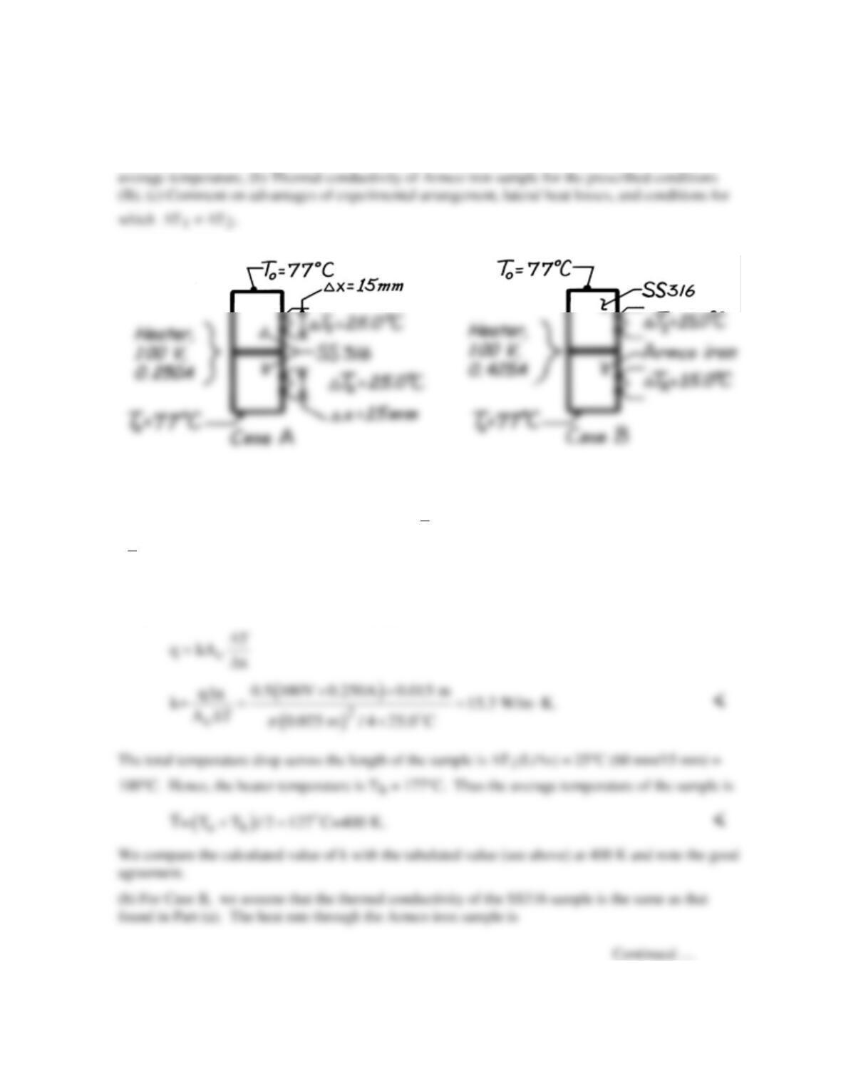
KNOWN: Electrical heater sandwiched between two identical cylindrical (25 mm dia. × 60 mm
length) samples whose opposite ends contact plates maintained at To.
FIND: (a) Thermal conductivity of SS316 samples for the prescribed conditions (A) and their
SCHEMATIC:
ASSUMPTIONS: (1) One-dimensional heat transfer in samples, (2) Steady–state conditions, (3)
Negligible contact resistance between materials.
PROPERTIES: Table A.2, Stainless steel 316
( )
ss
T=400 K : k 15.2 W/m K;= ⋅
Armco iron
( )
iron
T=380 K : k 67.2 W/m K.= ⋅
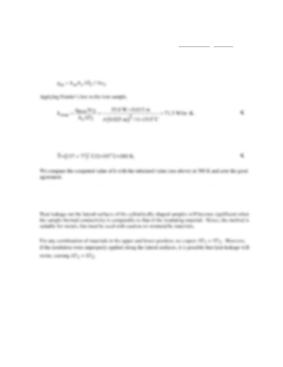
ANALYSIS: (a) For Case A recognize that half the heater power will pass through each of the
samples which are presumed identical. Apply Fourier’s law to a sample
PROBLEM 2.10 (Cont.)
( )
( )
2
iron heater ss
iron
0.025 m 15.0 C
q q q 100V 0.425A 15.3 W/m K 4 0.015 m
q 42.5 7.51 W= 35.0 W
π
= − = × − ⋅× ×
= −
where
The total drop across the iron sample is 15°C(60/15) = 60°C; the heater temperature is (77 + 60)°C =
137°C. Hence the average temperature of the iron sample is
(c) The principal advantage of having two identical samples is the assurance that all the electrical
power dissipated in the heater will appear as equivalent heat flows through the samples. With only
one sample, heat can flow from the backside of the heater even though insulated.
PROBLEM 2.11
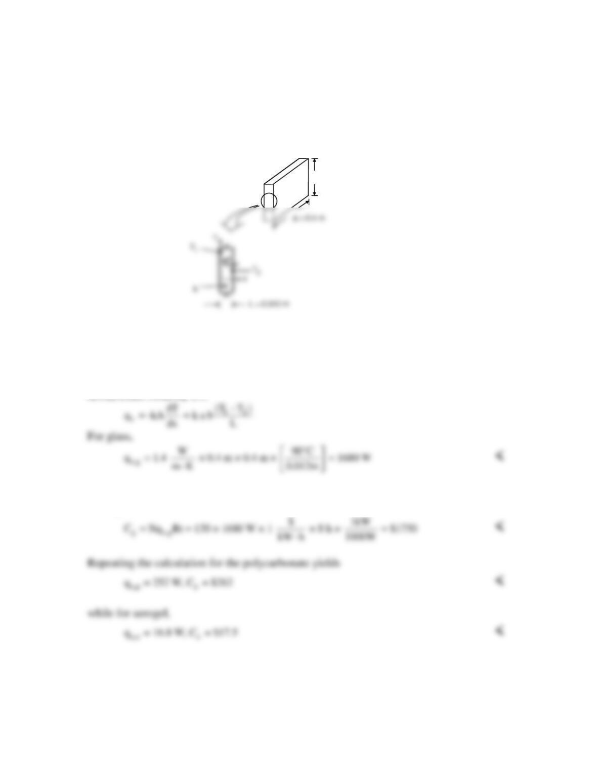
KNOWN: Dimensions of and temperature difference across an aircraft window. Window
materials and cost of energy.
FIND: Heat loss through one window and cost of heating for 130 windows on 8-hour trip.
SCHEMATIC:
ASSUMPTIONS: (1) Steady–state conditions, (2) One-dimensional conduction in the x-
direction, (3) Constant properties.
PROPERTIES: Table A.3, soda lime glass (300 K): kgl = 1.4 W/m⋅K.
ANALYSIS: From Eq. 2.1,
The cost associated with heat loss through N windows at a rate of R = $1/kW·h over a t =
8 h flight time is
COMMENT: Polycarbonate provides significant savings relative to glass. It is also lighter (ρp =
1200 kg/m3) relative to glass (ρg = 2500 kg/m3). The aerogel offers the best thermal performance
and is very light (ρa = 2 kg/m3) but would be relatively expensive.
b = 0.3 m
b = 0.3 m
b = 0.4 m
PROBLEM 2.12
KNOWN: Temperatures of various materials.
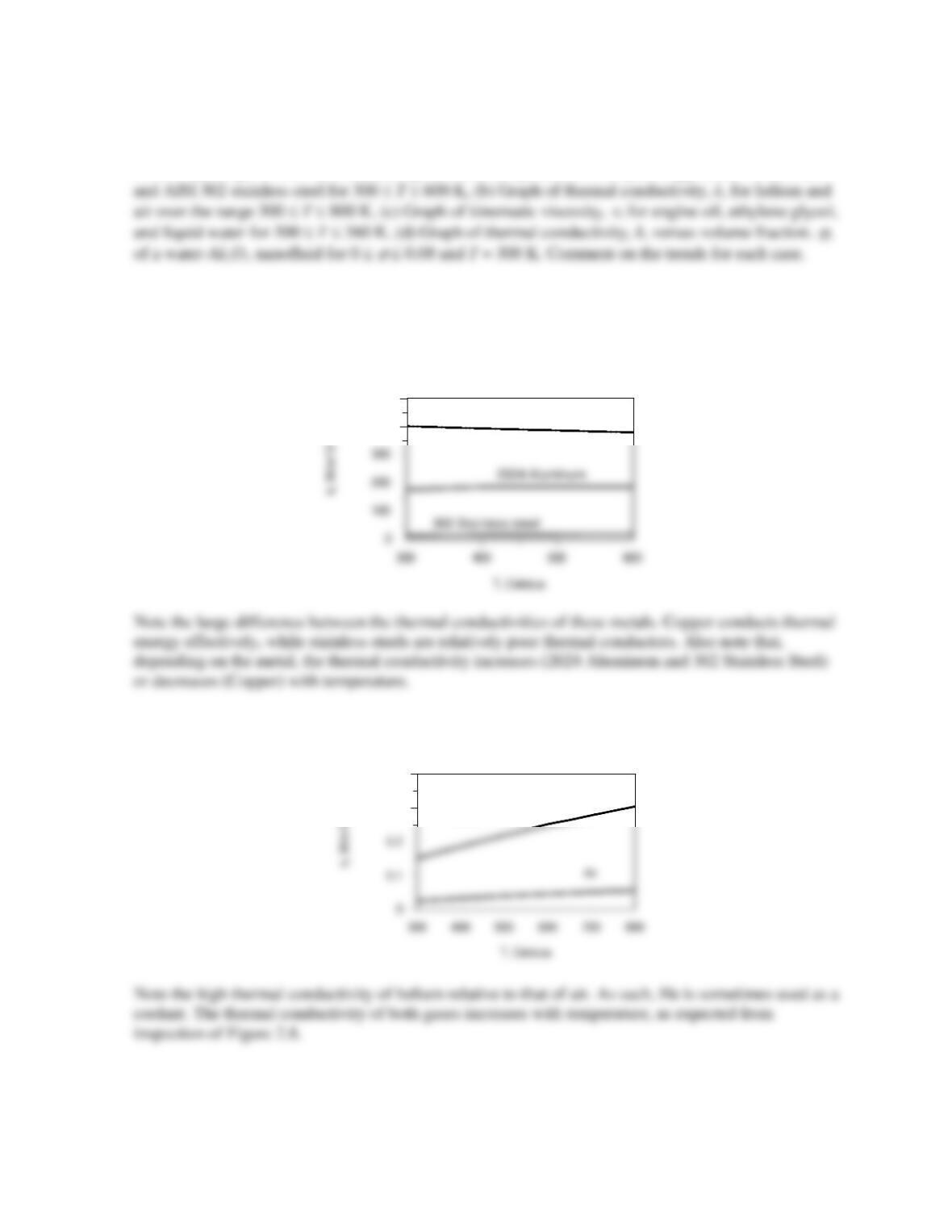
FIND: (a) Graph of thermal conductivity, k, versus temperature, T, for pure copper, 2024 aluminum
ASSUMPTION: (1) Constant nanoparticle properties.
ANALYSIS: (a) Using the IHT workspace of Comment 1 yields
(b) Using the IHT workspace of Comment 2 yields
Continued…
Thermal Conductivity of Cu, 2024 Al, and 302 ss
400
500
Copper
Thermal Conductivity of Helium and Air
0.3
0.4
Helium
PROBLEM 2.12 (Cont.)
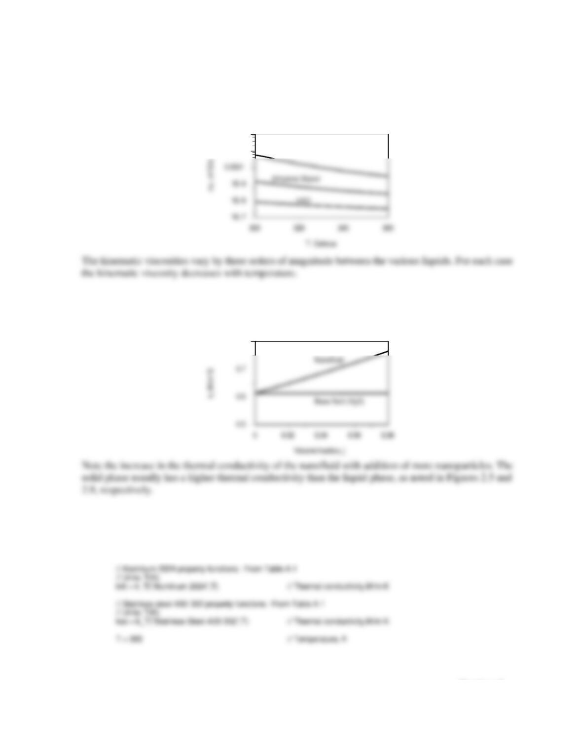
(c) Using the IHT workspace of Comment 3 yields
(d) Using the IHT workspace of Comment 4 yields
COMMENTS: (1) The IHT workspace for part (a) is as follows.
// Copper (pure) property functions : From Table A.1
// Units: T(K)
kCu = k_T(“Copper”,T) // Thermal conductivity,W/m·K
Continued…
Kinematic Viscosity of Eng ine Oil, Ethylene Glycol and H2O
0.001
0.01
Engine Oil
Thermal Conductivity of Nanofluid and Base Fluid
0.8
PROBLEM 2.12 (Cont.)
(2) The IHT workspace for part (b) follows.
// Helium property functions : From Table A.4
(3) The IHT workspace for part (c) follows.
// Engine Oil property functions : From Table A.5
// Units: T(K)
nuOil = nu_T(“Engine Oil”,T) // Kinematic viscosity, m^2/s
(4) The IHT workspace for part (d) follows.
// Water property functions :T dependence, From Table A.6
// Units: T(K), p(bars);
PROBLEM 2.13
KNOWN: Ideal gas behavior for air, hydrogen and carbon dioxide.
FIND: The thermal conductivity of each gas at 300 K. Compare calculated values to values from
Table A.4.
ASSUMPTIONS: (1) Ideal gas behavior.
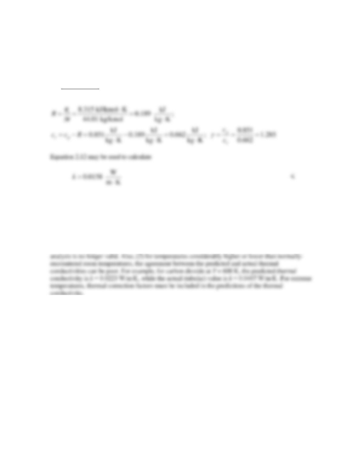
ANALYSIS: For air, the ideal gas constant, specific heat at constant volume, and ratio of specific
heats are:
From Equation 2.12
The thermal conductivity of air at T = 300 K is 0.0263 W/m∙K. Hence, the computed value is within 5
% of the reported value.
For hydrogen, the ideal gas constant, specific heat at constant volume, and ratio of specific heats are:
PROBLEM 2.13 (Cont.)
The thermal conductivity of hydrogen at T = 300 K is 0.183 W/m∙K. Hence, the computed value is
within 6 % of the reported value.
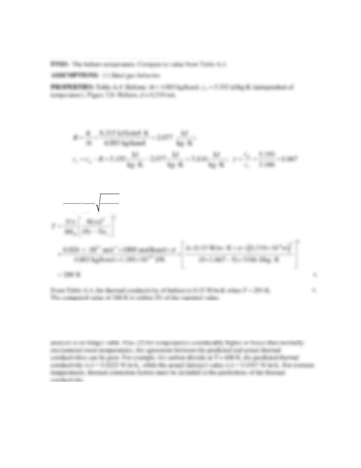
For carbon dioxide, the ideal gas constant, specific heat at constant volume, and ratio of specific heats
are:
The thermal conductivity of carbon dioxide at T = 300 K is 0.0166 W/m∙K. Hence, the computed
value is within 5 % of the reported value.
COMMENTS: The preceding analysis may be used to estimate the thermal conductivity at various
temperatures. However, the analysis is not valid for extreme temperatures or pressures. For example,
(1) the thermal conductivity is predicted to be independent of the pressure of the gas. As pure vacuum
conditions are approached, the thermal conductivity will suddenly drop to zero, and the preceding
PROBLEM 2.14
KNOWN: Thermal conductivity of helium.
ANALYSIS: For helium, the gas constant, specific heat at constant volume, and ratio of specific heats
are:
From Equation 2.12
2
95
4
vB
ckT
kd
g
ππ
−
=
M
N
COMMENTS: The preceding analysis may be used to estimate the thermal conductivity at various
temperatures. However, the analysis is not valid for extreme temperatures or pressures. For example,
(1) the thermal conductivity is predicted to be independent of the pressure of the gas. As pure vacuum
conditions are approached, the thermal conductivity will suddenly drop to zero, and the preceding