PROBLEM 2.41 (Cont.)
Substitute T(r) into the HDE to see if it is satisfied:
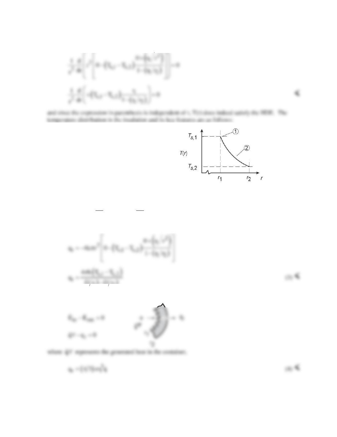
(1) Ts,1 > Ts,2
(2) Decreasing gradient with increasing radius,
r, since the heat rate is constant through
the insulation.
(b) Using Fourier’s law for the radial-spherical coordinate, the heat rate through the insulation is
()
2
rr
dT dT
q kA k 4 r
dr dr
π
=−=−
<
and substituting for the temperature distribution, Eq. (2),
( ) ( )
12
Applying an energy balance to a control surface about the container at r = r1,
Continued…
PROBLEM 2.41 (Cont.)
(c) Applying an energy balance to a control surface placed around the outer surface of the insulation,
These relations can be used to determine Ts,2 in terms of the variables
q
“
, r1, r2, h,
T
∞
, ε and Tsur.
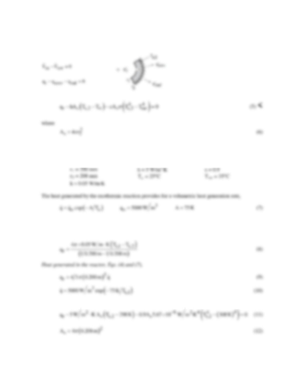
(d) Consider the reactor system operating under the following conditions:
where the temperature of the reaction is that of the inner surface of the insulation, To = Ts,1. The
following system of equations will determine the operating conditions for the reactor.
Conduction rate equation, insulation, Eq. (3),
Surface energy balance, insulation, Eqs. (5) and (6),
Continued…
PROBLEM 2.41 (Cont.)
Solving these equations simultaneously, find that
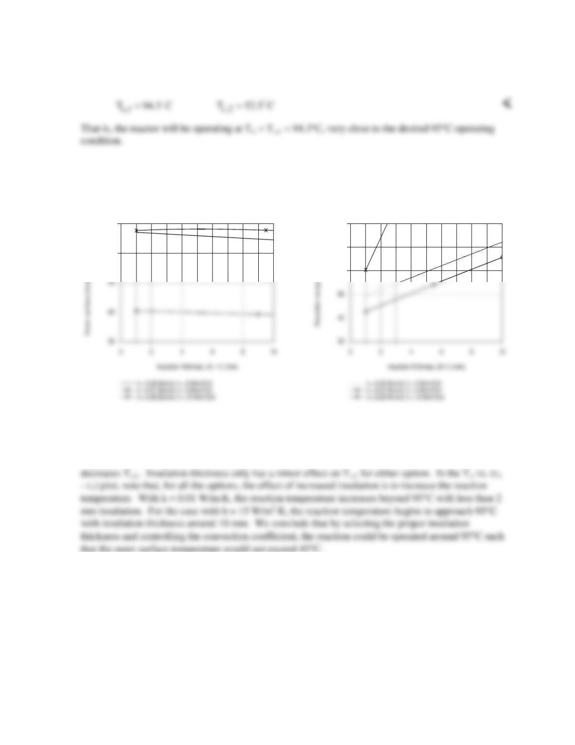
(e) Using the above system of equations, Eqs. (8)-(12), we have explored the effects of changes in the
convection coefficient, h, and the insulation thermal conductivity, k, as a function of insulation
thickness, t = r2 – r1.
50
55
80
100
120
In the Ts,2 vs. (r2 – r1) plot, note that decreasing the thermal conductivity from 0.05 to 0.01 W/m⋅K
slightly increases Ts,2 while increasing the convection coefficient from 5 to 15 W/m2⋅K markedly
PROBLEM 2.42
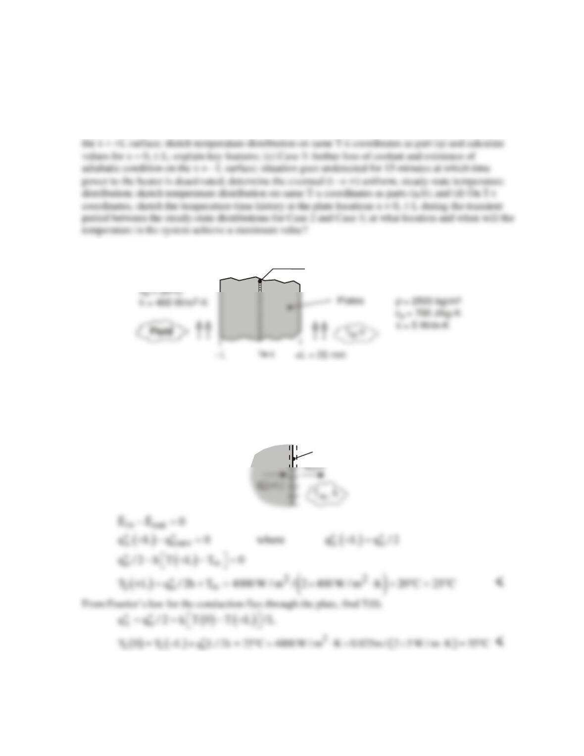
KNOWN: Thin electrical heater dissipating 4000 W/m2 sandwiched between two 25-mm thick plates
whose surfaces experience convection.
FIND: (a) On T–x coordinates, sketch the steady–state temperature distribution for –L ≤ × ≤ +L;
calculate values for the surfaces x = L and the mid–point, x = 0; label this distribution as Case 1 and
explain key features; (b) Case 2: sudden loss of coolant causing existence of adiabatic condition on
SCHEMATIC:
Electric heater
q” = 4000 W/m
2
o
o
ASSUMPTIONS: (1) One–dimensional conduction, (2) Constant properties, (3) No internal
volumetric generation in plates, and (3) Negligible thermal resistance between the heater surfaces and
the plates.
ANALYSIS: (a) Since the system is symmetrical, the heater power results in equal conduction fluxes
through the plates. By applying a surface energy balance on the surface x = +L as shown in the
schematic, determine the temperatures at the mid–point, x = 0, and the exposed surface, x + L.
T(+L)
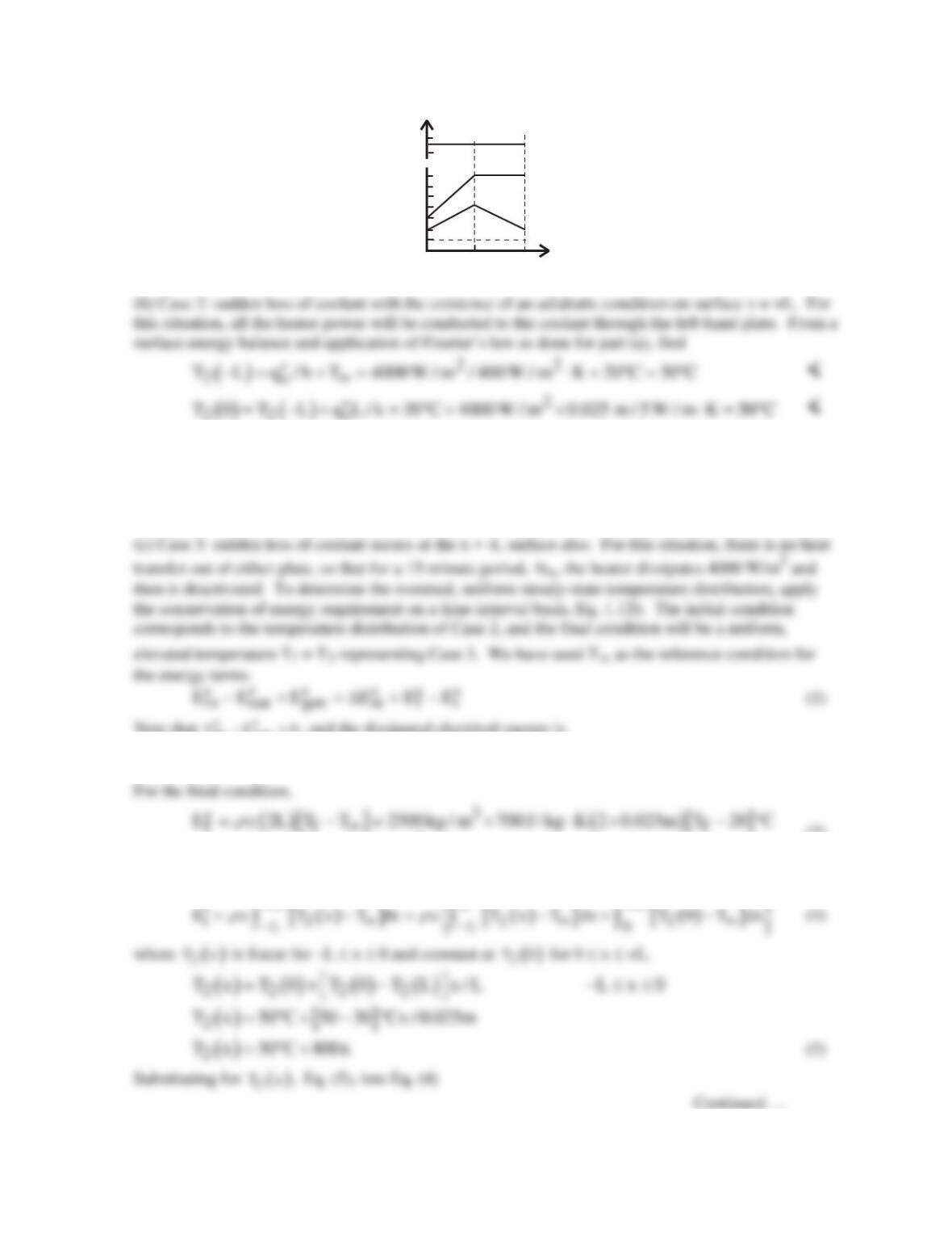
The temperature distribution is shown on the T-x coordinates below and labeled Case 1. The key
features of the distribution are its symmetry about the heater plane and its linear dependence with
distance.
Continued …
PROBLEM 2.42 (Cont.)
T(x), ( C)
o
0x
-L +L
50
30
40
86.1
T (0) = 35 C
1o
Case 1, T (x)
1
Case 2, T (x)
2
Case 3, T (x)
3
= 20
T
o
o
The temperature distribution is shown on the T-x coordinates above and labeled Case 2. The
distribution is linear in the left–hand plate, with the maximum value at the mid-point. Since no heat
flows through the right-hand plate, the gradient must zero and this plate is at the maximum
temperature as well. The maximum temperature is higher than for Case 1 because the heat flux
through the left-hand plate has increased two-fold.
Note that
in out
EE 0
−=
, and the dissipated electrical energy is
( )
2 62
gen o o
E q t 4000 W / m 15 60 s 3.600 10 J / m
′′ ′′
=∆= × = ×
(2)
[ ]
42
ff
8.75 10 T 20 J / m
E
=×−
′′
(3)
where Tf = T3, the final uniform temperature, Case 3. For the initial condition,
PROBLEM 2.42 (Cont.)
i
Returning to the energy balance, Eq. (1), and substituting Eqs. (2), (3) and (6), find Tf = T3.
[ ]
62 4 62
3
3.600 10 J / m 8.75 10 T 20 2.188 10 J / m× = × −− ×
( )
3
T 66.1 20 C 86.1 C= + °= °
<
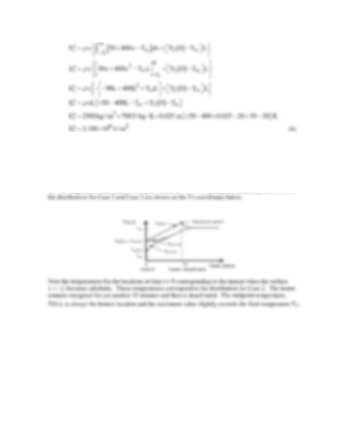
The temperature distribution is shown on the T-x coordinates above and labeled Case 3. The
distribution is uniform, and considerably higher than the maximum value for Case 2.
(d) The temperature–time history at the plate locations x = 0, ± L during the transient period between
PROBLEM 2.43
KNOWN: Plane wall, initially at a uniform temperature, is suddenly exposed to convective heating.
FIND: (a) Differential equation and initial and boundary conditions which may be used to find the
temperature distribution, T(x,t); (b) Sketch T(x,t) for these conditions: initial (t ≤ 0), steady-state, t →
∞, and two intermediate times; (c) Sketch heat fluxes as a function of time for surface locations; (d)
Expression for total energy transferred to wall per unit volume (J/m3).
ASSUMPTIONS: (1) One-dimensional conduction, (2) Constant properties, (3) No internal heat
generation.
ANALYSIS: (a) For one-dimensional conduction with constant properties, the heat equation has the
form,
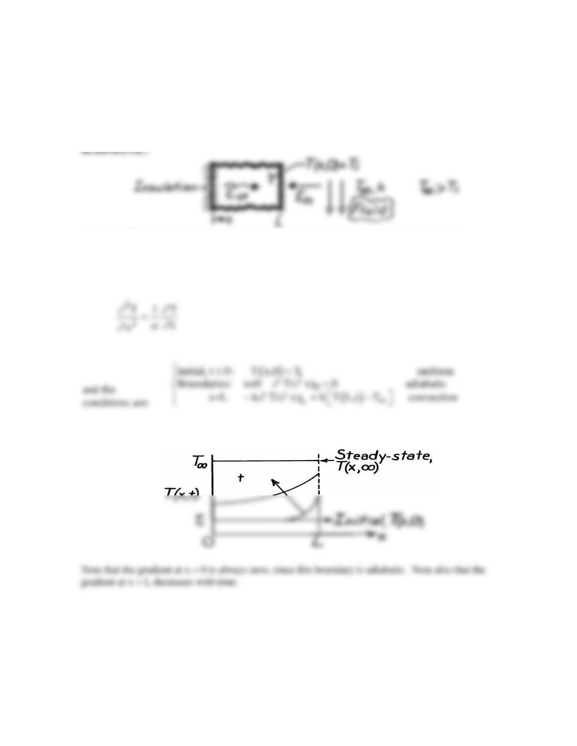
(b) The temperature distributions are shown on the sketch.
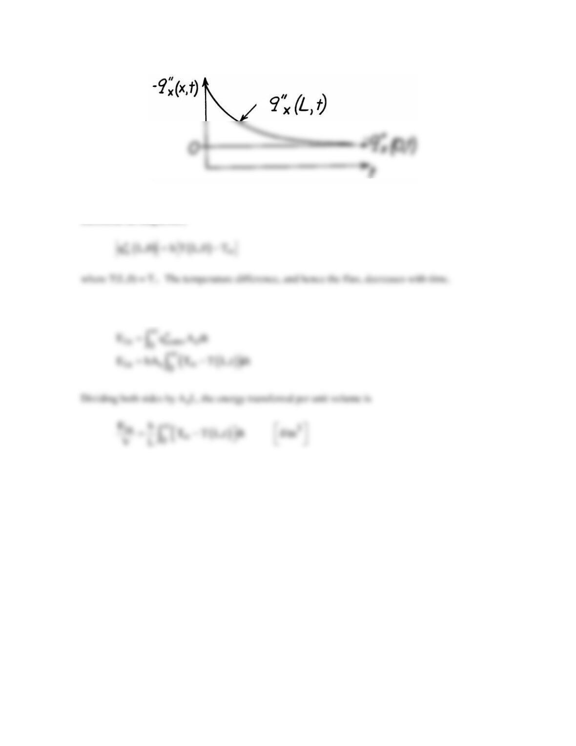
(c) The heat flux,
( )
x
q x,t ,
′′
as a function of time, is shown on the sketch for the surfaces x = 0 and x
= L.
Continued …
PROBLEM 2.43 (Cont.)
For the surface at
( )
x
x 0, q 0, t 0
′′
= =
since it is adiabatic. At x = L and t = 0,
( )
x
q L,0
′′
is a
maximum (in magnitude)
(d) The total energy transferred to the wall may be expressed as
COMMENTS: Note that the heat flux at x = L is into the wall and is hence in the negative x
direction.
–
–
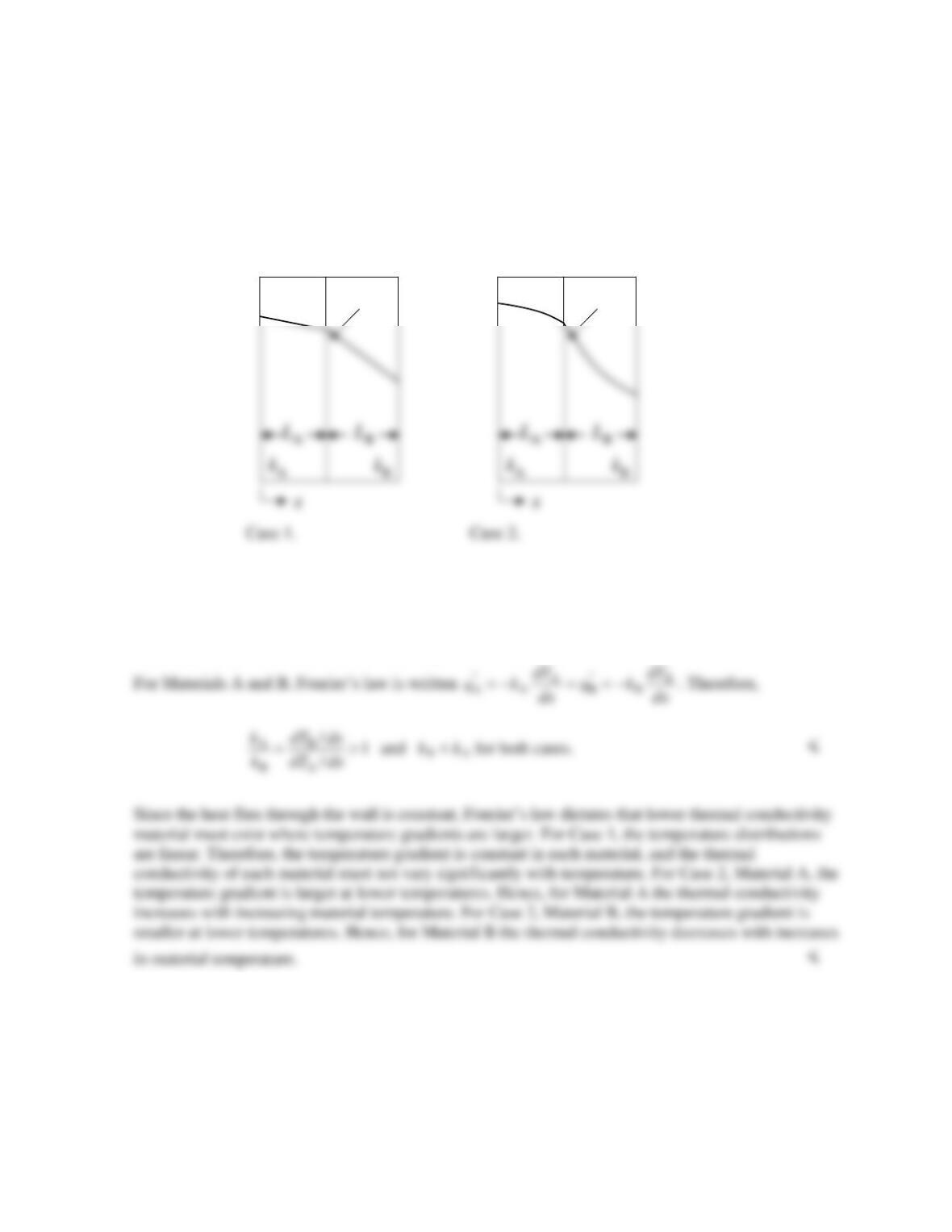
PROBLEM 2.44
KNOWN: Qualitative temperature distributions in two cases.
FIND: For each of two cases, determine which material (A or B) has the higher thermal conductivity,
how the thermal conductivity varies with temperature, description of the heat flux distribution through
the composite wall, effect of simultaneously doubling the wall thickness and thermal conductivity.
SCHEMATIC:
ASSUMPTIONS: (1) Steady–state, one–dimensional conditions, (2) Negligible contact resistances,
(3) No internal energy generation.
ANALYSIS: Under steady-state conditions with no internal generation, the conservation of energy
requirement dictates that the heat flux through the wall must be constant. <
COMMENTS: If you were given information regarding the relative values of the thermal
conductivities and how the thermal conductivities vary with temperature in each material, you should
be able to sketch the temperature distributions provided in the problem statement.
T(x)
T(x)
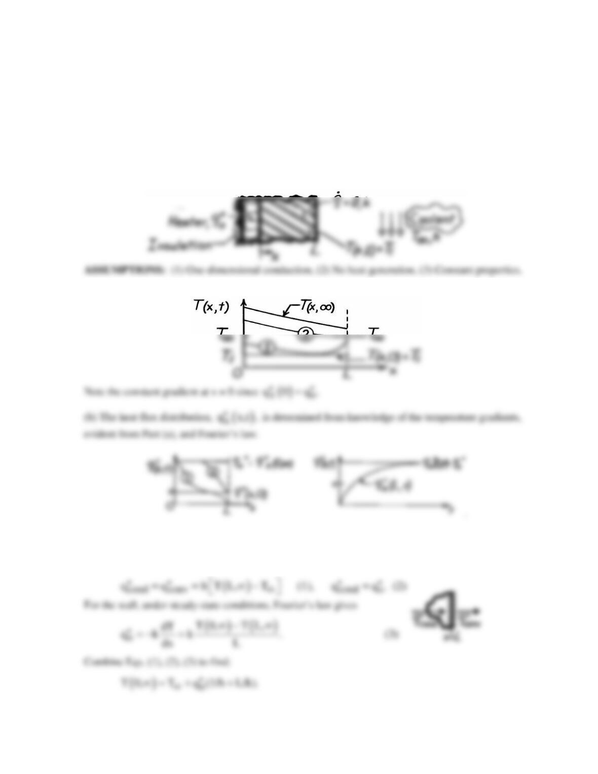
PROBLEM 2.45
KNOWN: Plane wall, initially at a uniform temperature Ti, is suddenly exposed to convection with a
fluid at T∞ at one surface, while the other surface is exposed to a constant heat flux
′′
q
o
.
FIND: (a) Temperature distributions, T(x,t), for initial, steady-state and two intermediate times, (b)
Corresponding heat fluxes on
′′ −q x
x
coordinates, (c) Heat flux at locations x = 0 and x = L as a
function of time, (d) Expression for the steady-state temperature of the heater, T(0,∞), in terms of
′′
∞
q T k, h and L.
o
, ,
SCHEMATIC:
ANALYSIS: (a) For
T T
i
<
∞
,
the temperature distributions are
(c) On
( )
x
q x,t t
′′ −
coordinates, the heat fluxes at the boundaries are shown above.
(d) Perform a surface energy balance at x = L and an energy balance on the wall:
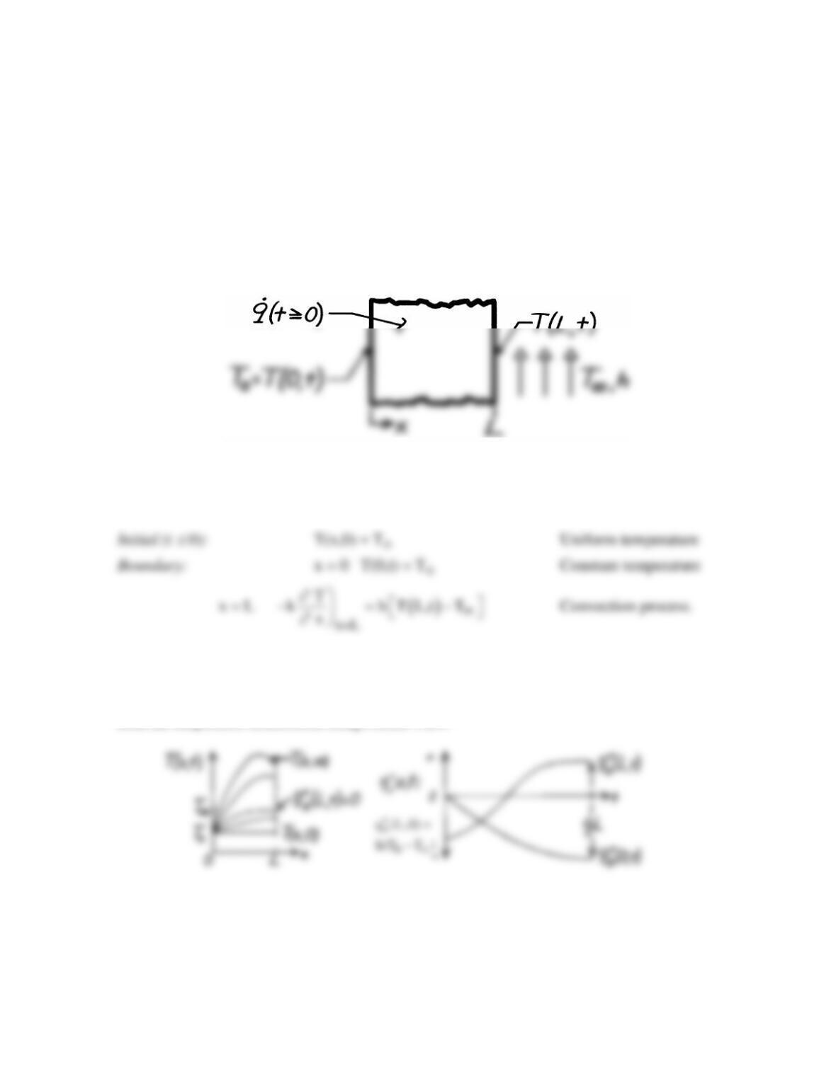
PROBLEM 2.46
KNOWN: Plane wall, initially at a uniform temperature To, has one surface (x = L) suddenly
exposed to a convection process (T∞ > To,h), while the other surface (x = 0) is maintained at To.
Also, wall experiences uniform volumetric heating
“
q
such that the maximum steady–state temperature
will exceed T∞.
FIND: (a) Sketch temperature distribution (T vs. x) for following conditions: initial (t ≤ 0), steady-
state (t → ∞), and two intermediate times; also show distribution when there is no heat flow at the x =
L boundary, (b) Sketch the heat flux
( )
x
q vs. t
′′
at the boundaries x = 0 and L.
SCHEMATIC:
ASSUMPTIONS: (1) One-dimensional conduction, (2) Constant properties, (3) Uniform volumetric
generation, (4)
T T and q
o
<
∞
“
large enough that T(x,∞) > T∞ for some x.
ANALYSIS: (a) The initial and boundary conditions for the wall can be written as
The temperature distributions are shown on the T-x coordinates below. Note the special condition
when the heat flux at (x = L) is zero.
(b) The heat flux as a function of time at the boundaries,
( ) ( )
xx
q 0, t and q L,t ,
′′ ′′
can be inferred
from the temperature distributions using Fourier’s law.
COMMENTS: Since
( )
o
T x, T for some x and T T ,
∞∞
∞> >
heat transfer at both boundaries must be
out of the wall at steady state. From an overall energy balance at steady state,
( ) ( )
xx
q L, q 0, qL.
′′ ′′
+ ∞− ∞
=
“
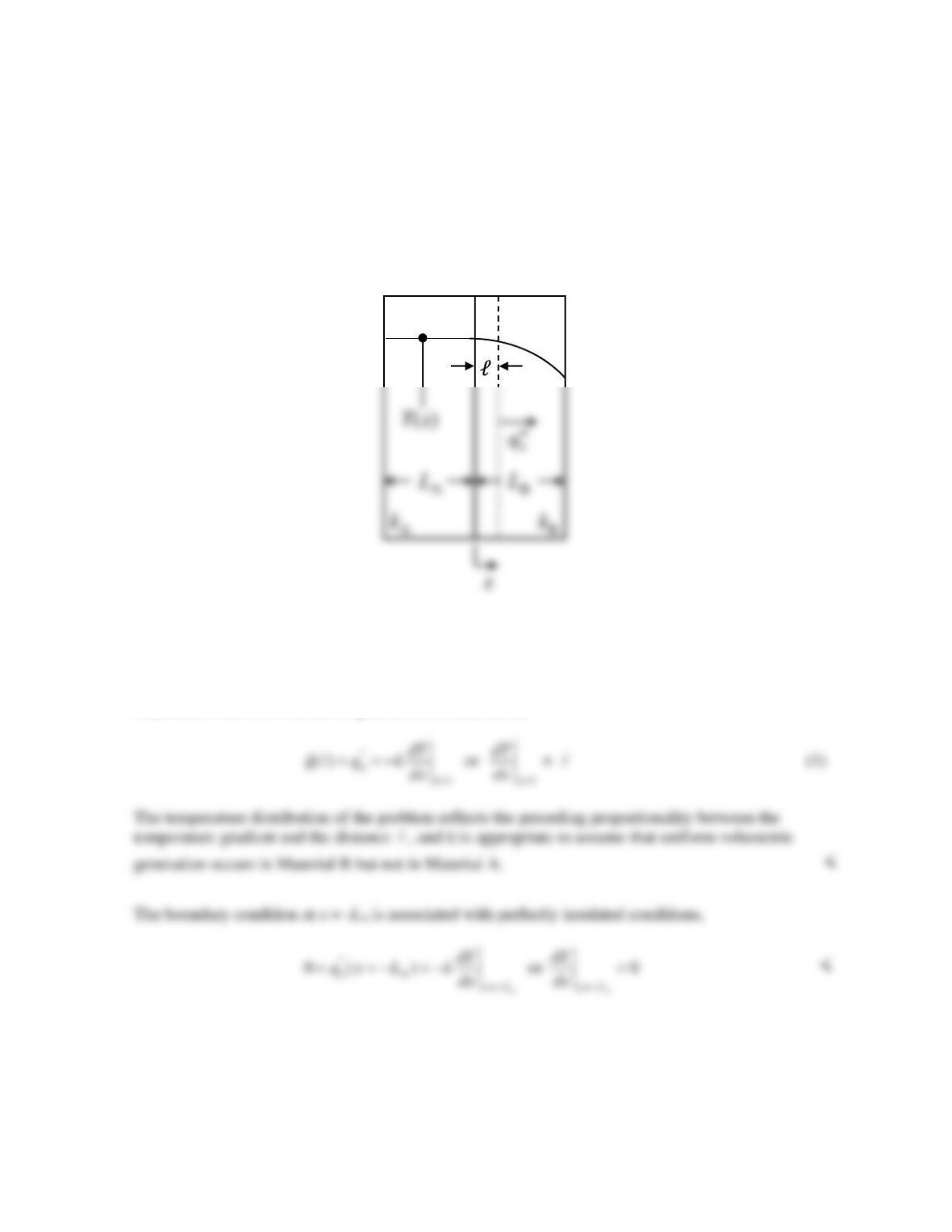
PROBLEM 2.47
KNOWN: Qualitative temperature distribution in a composite wall with one material experiencing
uniform volumetric energy generation.
FIND: Which material experiences uniform volumetric generation. The boundary condition at
x = –LA. Temperature distribution if the thermal conductivity of Material A is doubled. Temperature
distribution if the thermal conductivity of Material B is doubled. Sketch the heat flux distribution
“
()
x
qx
through the composite wall.
SCHEMATIC:
ASSUMPTIONS: (1) Steady–state, one–dimensional conditions, (2) Constant properties.
ANALYSIS: Consider a control volume with the LHS control surface at the interface between the
two materials and the RHS control surface located at an arbitrary location within Material B, as shown
in the schematic. For this control volume, conservation of energy and Fourier’s law may be combined
to yield, for uniform volumetric generation in Material B,
The temperature distribution in Material A corresponds to
“
,A
0
x
q=
, and is independent of its thermal
conductivity. <
Continued…