Appendix 19
A19.1 t-estimator of µ
n
s
tx 2/
1
2
3
A B C D
t-Estimate: Mean
Plastic bags
A19.2 Spearman rank correlation coefficient test
H0: ρS = 0
H1: ρS > 0
1nrz S−=
1
2
3
A B C D
Spearman Rank Correlation
Satisfaction and Time
A19.3 Sign test
H0: The location of the two populations are the same
1
2
3
4
A B C D E
Sign Test
Difference Cork rate – Metal rate
A19.4 Histograms (not shown) are approximately bell shaped
Unequal-variances t-test of
21 −
)(:H 210 −
= 0
1
2
3
4
5
A B C
t-Test: Two-Sample Assuming Unequal Variances
British American
Mean 7137 9304
Variance 38051 110151
A19.5 Spearman rank correlation coefficient test
H0: ρS = 0
H1: ρS > 0
1nrz S−=
1
2
3
A B C D
Spearman Rank Correlation
Parking and Visits
A19.6 t-test of ρ or β1
:H
0
= 0
0:H1
2
r1
2n
rt −
−
=
1
2
3
A B
Correlation
Visits and Income
A19.7 Histograms of Groups 1 and 2: Interpersonal
50
100
Histogram: Group 1 Interpersonal
50
100
Histogram: Group2 Interpersonal
The histograms indicate that the scores are extremely nonnormal.
Interpersonal skills: Wilcoxon rank sum test
H0: The two population locations are the same
H1: The location of population 1 is to the right of the location of population 2
1
2
3
4
A B C D
Wilcoxon Rank Sum Test
Rank Sum Observations
Gp 1 Interpersonal 36392 187
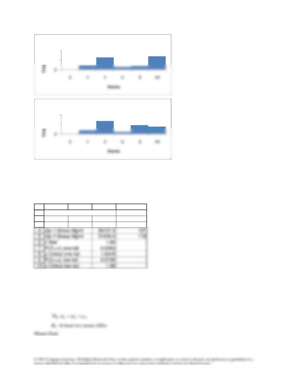
Histograms of Groups 1 and 2: Stress Management
50
100
Histogram: Group 1 Stress Management
50
100
Histogram: Group 2 Stress Management
The histograms indicate that the scores are extremely nonnormal.
Stress management: Wilcoxon rank sum test
H0: The two population locations are the same
H1: The location of population 1 is to the right of the location of population 2
1
2
3
A B C D
Wilcoxon Rank Sum Test
Rank Sum Observations
z = 1.80; p-value = .0363. There is enough evidence to conclude that students whose university GPA is greater than
3.0 score higher on stress management than students whose university GPA is less than 2.
A19.8 All histograms (not shown) are somewhat bell shaped.
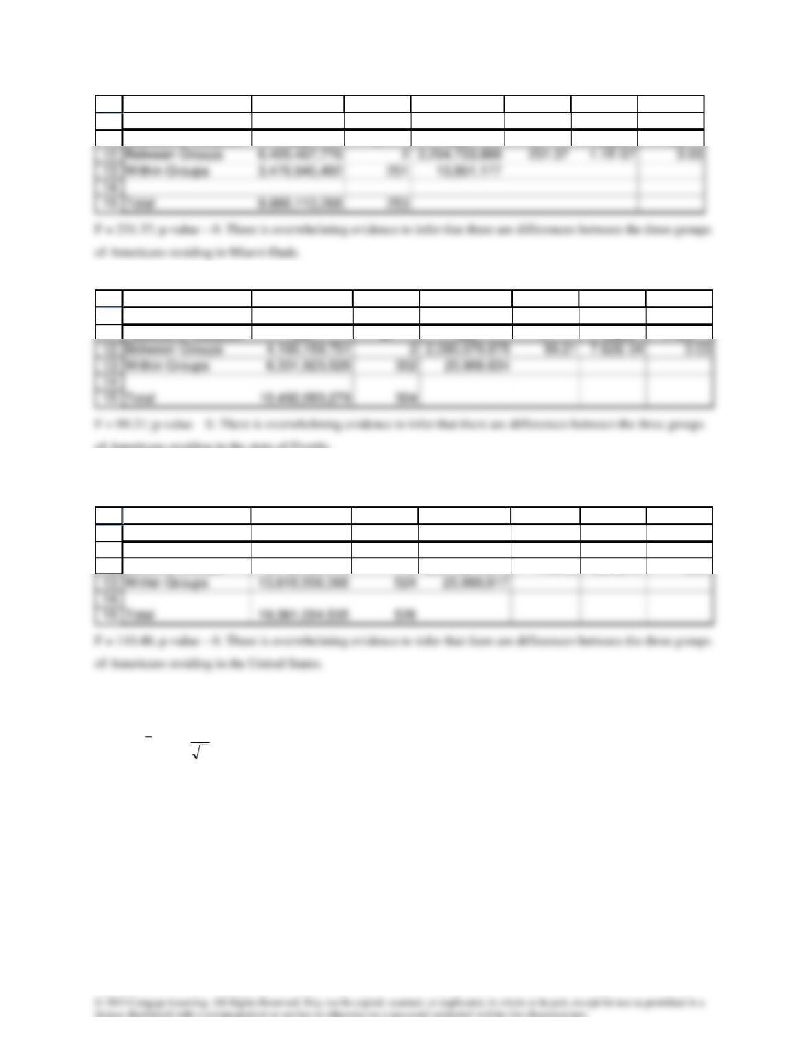
One-way analysis of variance
10
15
11
A B C D E F G
ANOVA
Source of Variation SS df MS F P-value F crit
Florida
10
15
11
A B C D E F G
ANOVA
Source of Variation SS df MS F P-value F crit
of Americans residing in the state of Florida.
United States
10
11
12
A B C D E F G
ANOVA
Source of Variation SS df MS F P-value F crit
Between Groups 5,742,495,149 2 2,871,247,574 110.48 9.27E-41 3.01
A19.9 t-estimator of µ
n
s
tx 2/
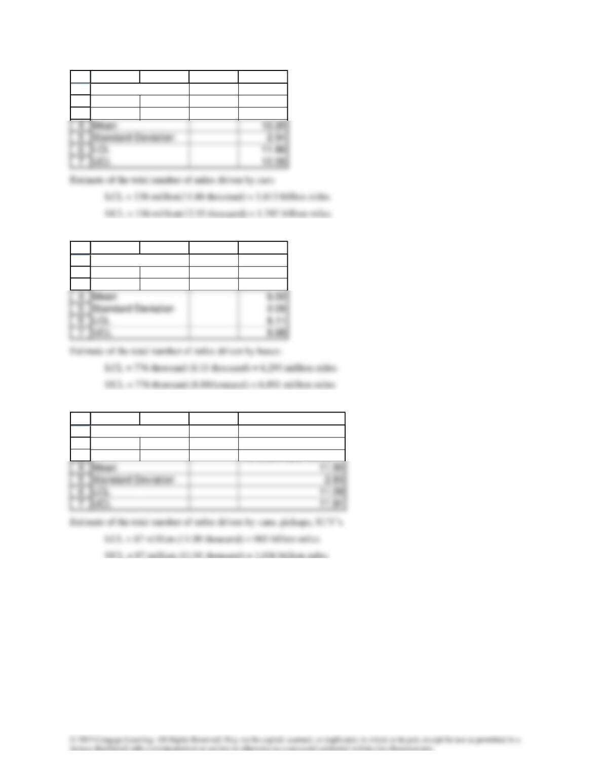
Cars
1
2
3
A B C D
t-Estimate: Mean
Cars
Buses
1
2
3
A B C D
t-Estimate: Mean
Buses
Vans, pickups, SUV’s
1
2
3
A B C D
t-Estimate: Mean
Vans, pickups, SUVs
UCL = 87 million (11.91 thousand) = 1,036 billion miles
A19.10 All three histograms (not shown) are bell shaped.
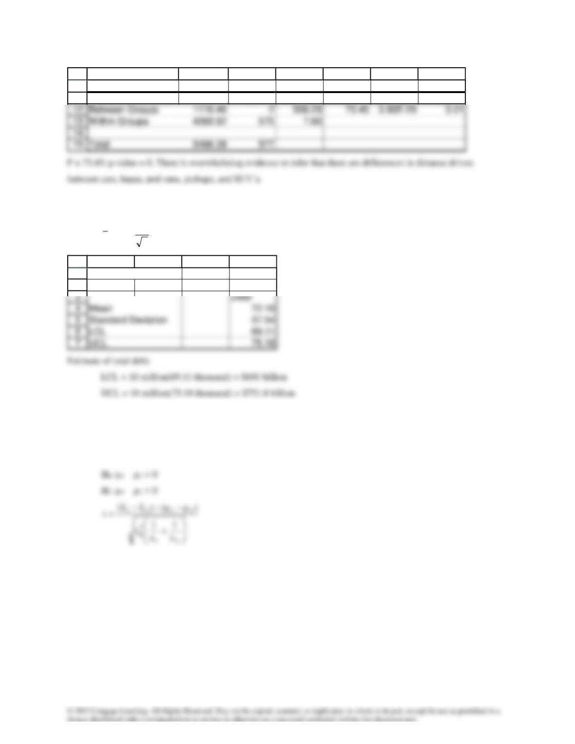
One-way analysis of variance
3210 :H ==
H1: At least two means differ
10
15
11
A B C D E F G
ANOVA
Source of Variation SS df MS F P-value F crit
A19.11 t-estimator of µ
n
s
tx 2/
1
2
A B C D
t-Estimate: Mean
A19.12 Both histograms (not shown) are positively skewed but not sufficiently so to violate the normality
requirement of the t-test of µ1 − µ2.
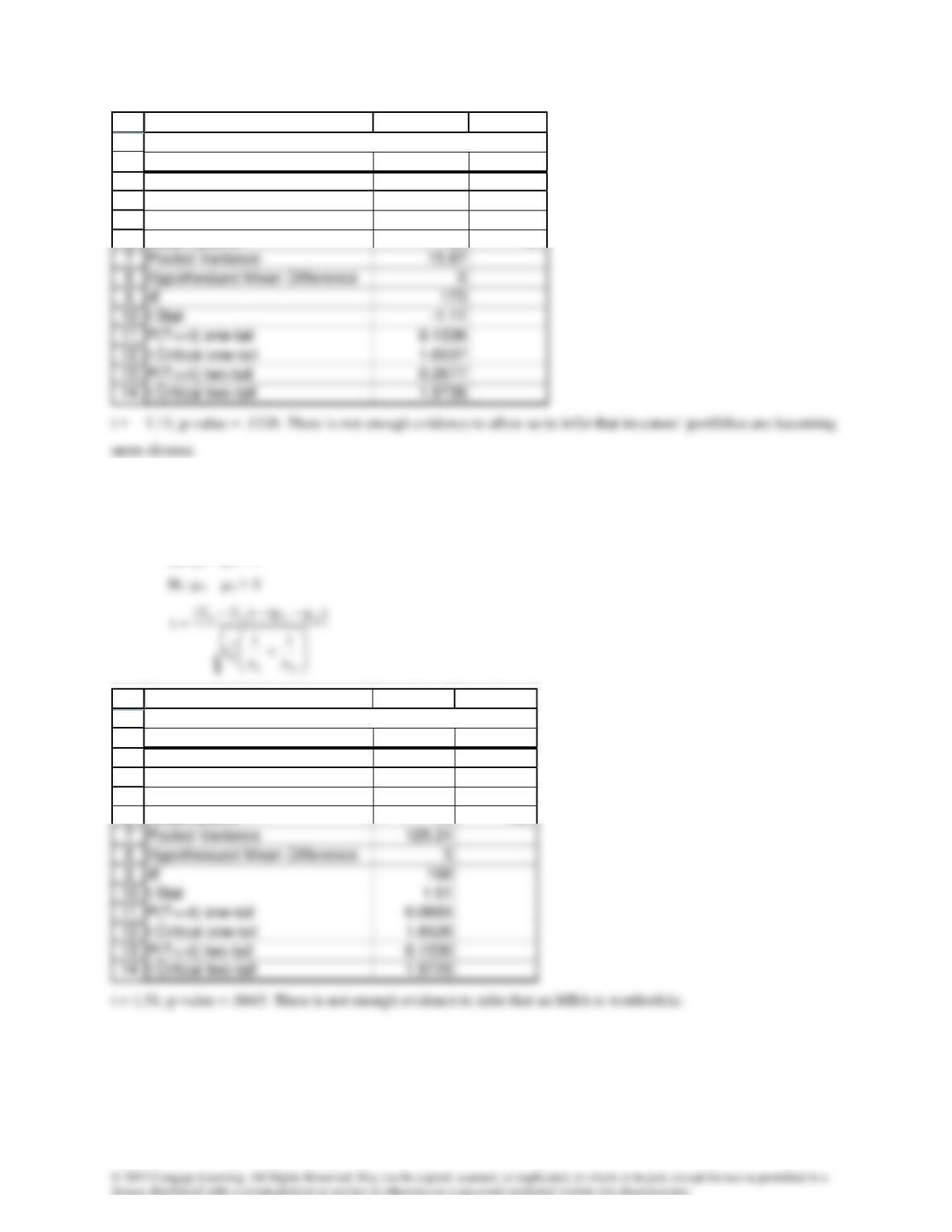
Equal-variances t-test of µ1 − µ2
1
2
3
4
5
6
A B C
t-Test: Two-Sample Assuming Equal Variances
5 years ago This year
Mean 7.14 7.81
Variance 12.87 18.64
Observations 84 91
A19.13 Both histograms (not shown) are bell shaped.
Equal-variances t-test of µ1 − µ2
H0: µ1 – µ2 = 5
1
2
3
4
5
6
A B C
t-Test: Two-Sample Assuming Equal Variances
MBA BBA
Mean 96.53 89.08
Variance 156.70 106.44
Observations 79 121
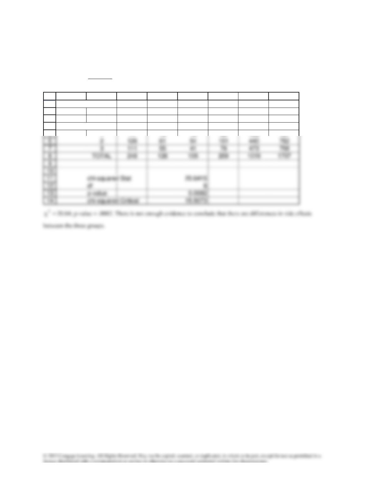
A19.14 Chi-squared test of a contingency table
:H0
The two variables are independent
:H1
The two variables are dependent
=
−
=
15
1i i
2
ii
2
e
)ef(
1
2
3
4
A B C D E F G H
Contingency Table
Group
Side Effect 1 2 3 4 5 TOTAL
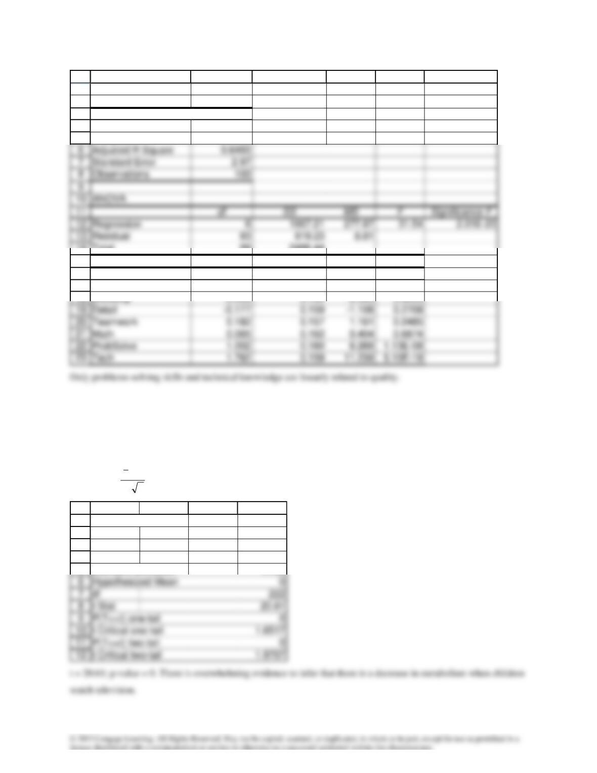
A19.15 Multiple regression
1
2
8
10
3
4
5
14
15
16
17
A B C D E F
SUMMARY OUTPUT
Regression Statistics
Multiple R 0.8189
R Square 0.6705
Total 99 2486.44
Coefficients Standard Error t Stat P-value
Intercept 1.005 1.387 0.725 0.4704
A19.16 a t-test of
=:H0
0
:H1
> 0
n/s
x
t−
=
1
2
3
4
5
A B C D
t-Test: Mean
Decrease
Mean 24.73
Standard Deviation 17.92
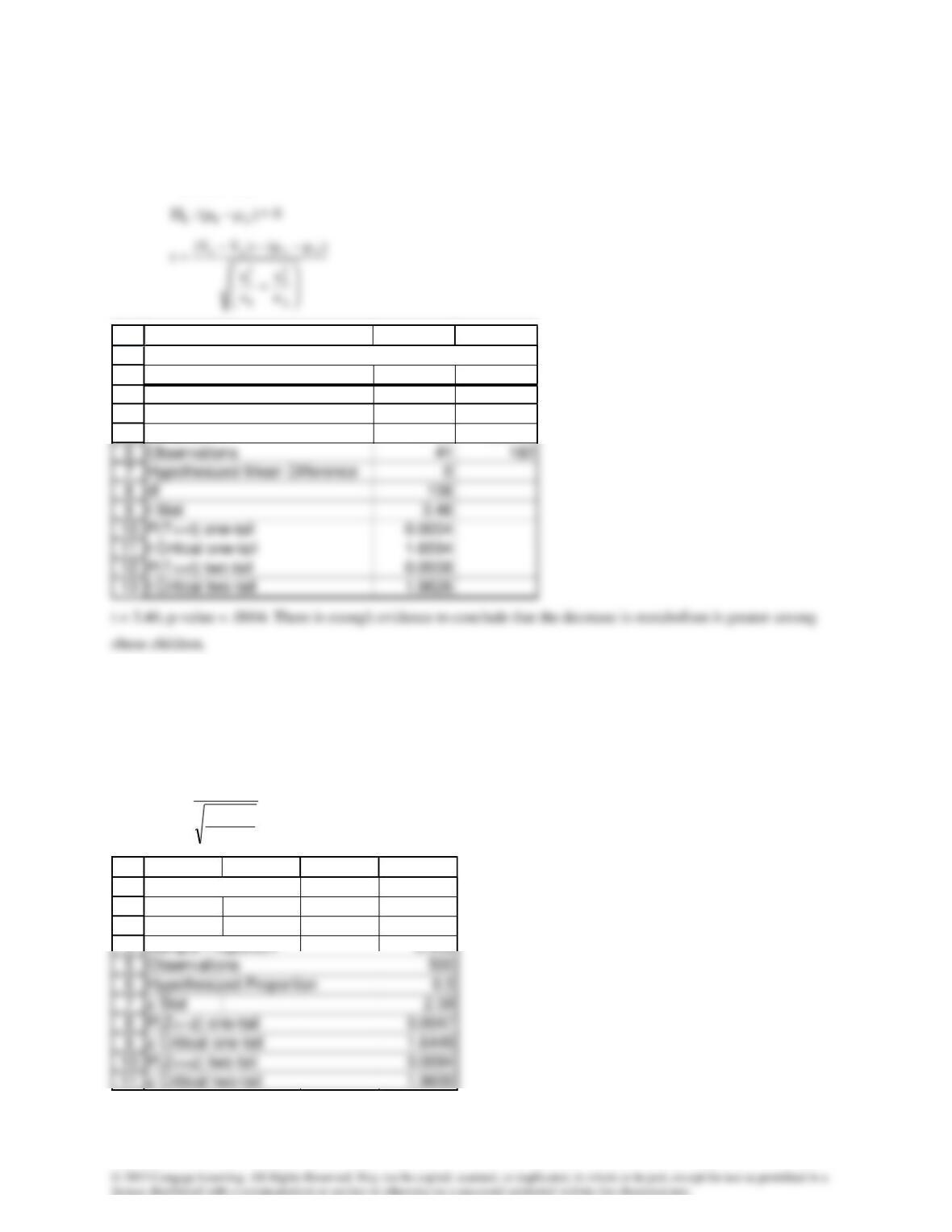
b Both histograms (not shown) are roughly bell shaped.
Unequal-variances t-test of
21 −
)(:H 210 −
= 0
1
2
3
4
5
A B C
t-Test: Two-Sample Assuming Unequal Variances
Obese Nonobese
Mean 30.86 23.35
Variance 112.85 358.58
A19.17 a z-test of p (success = mathematics major wins)
:H0
p = .5
:H1
p > .5
n
)p1(p
pp
ˆ
z−
−
=
1
2
3
A B C D
z-Test: Proportion
Math win
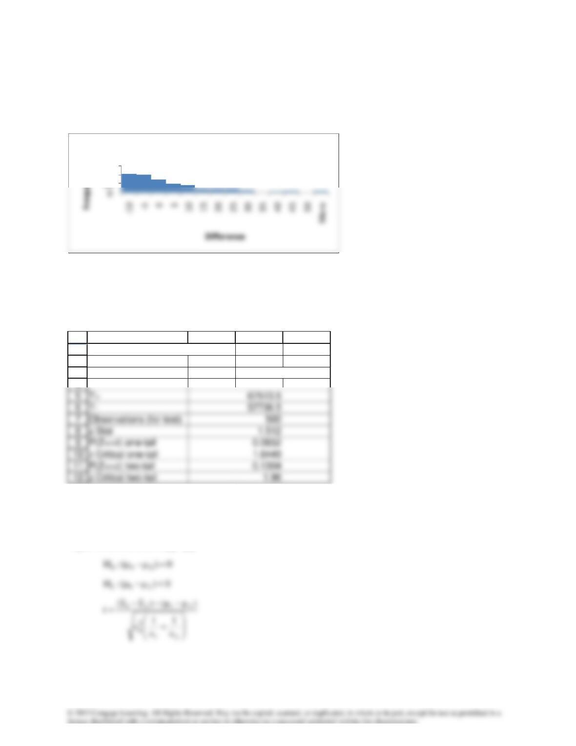
z = 2.59; p-value = .0047. There is enough evidence to infer that mathematics majors win more frequently than
English majors.
b Histogram of differences
100
150
Histogram
The matched pairs differences are extremely nonnormal.
Wilcoxon signed rank sum test
0
H
: The two population locations are the same.
:H1
The location of population 1 is to the right of the location of population 2.
1
2
3
A B C D
Wilcoxon Signed Rank Sum Test
Difference English – Math
z = 1.512, p-value = .0652. There is not enough evidence to infer that English majors outscore mathematics majors.
c Part (a) ignores the magnitude of the paired differences.
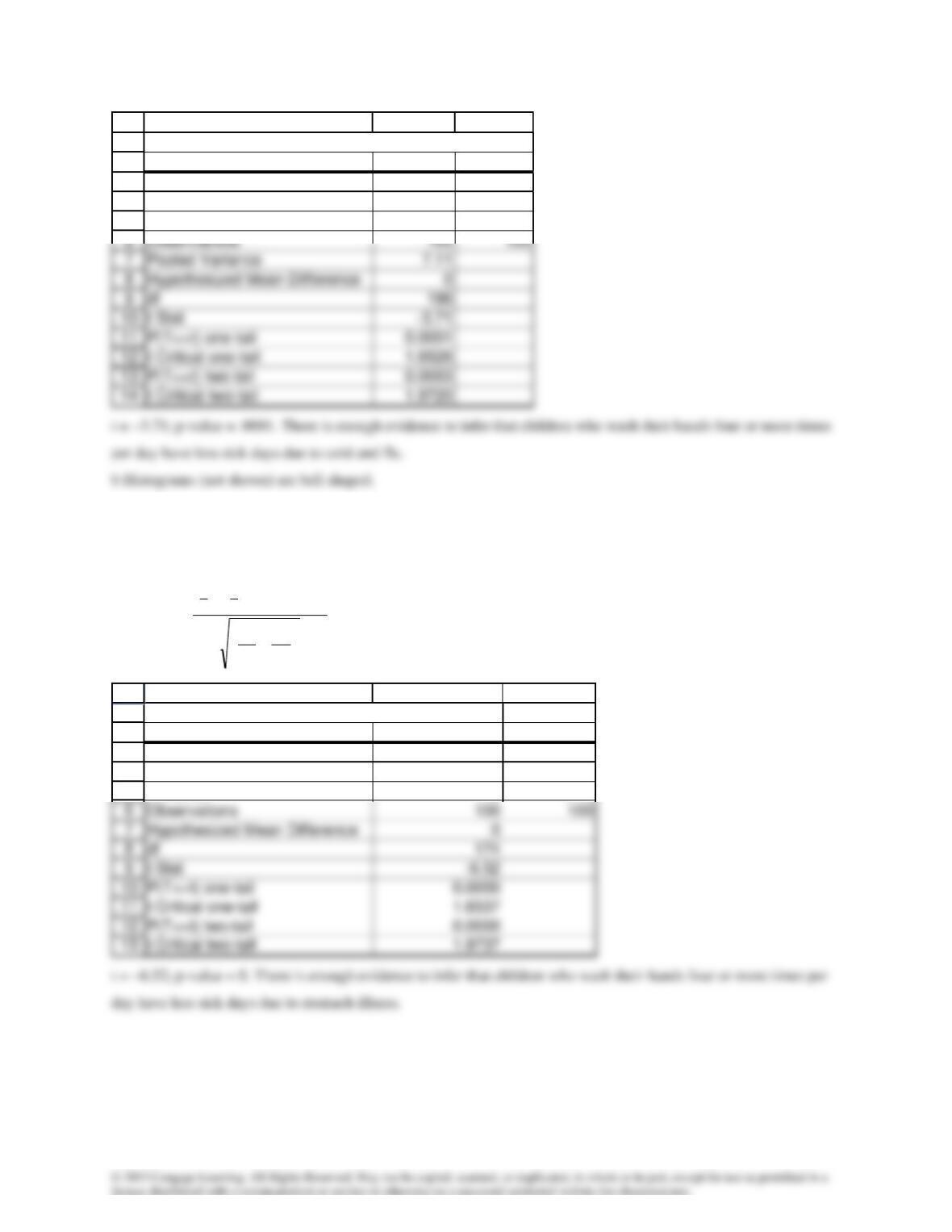
A19.18a Histograms (not shown) are bell shaped.
Equal-variances t-test of
21 −
1
2
3
4
5
A B C
t-Test: Two-Sample Assuming Equal Variances
4 or more Less
Mean 6.00 7.40
Variance 5.62 8.61
Unequal-variances t-test of
21 −
0)(:H 210 =−
)(:H 211 −
< 0
+
−−−
=
2
2
2
1
2
1
2121
n
s
n
s
)()xx(
t
1
2
3
4
5
A B C
t-Test: Two-Sample Assuming Unequal Variances
Four or more Less
Mean 1.76 3.17
Variance 1.48 3.19
A19.19 Spearman rank correlation coefficient test
H0: ρS = 0
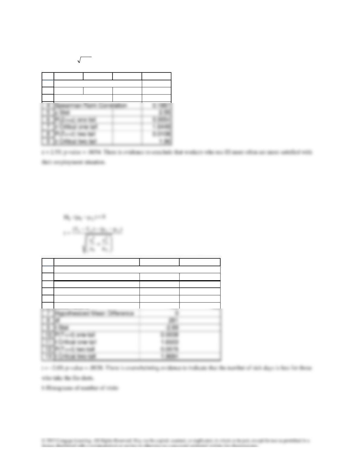
H1: ρS > 0
1nrz S−=
1
2
3
A B C D
Spearman Rank Correlation
EI and Satisfaction
A19.20 a Histograms (not shown) of sick days are bell shaped.
Unequal-variances t-test of
21 −
0)(:H 210 =−
1
2
3
4
5
6
A B C
t-Test: Two-Sample Assuming Unequal Variances
Days flu shot Days placebo
Mean 2.82 3.22
Variance 1.25 2.07
Observations 150 150
100
150
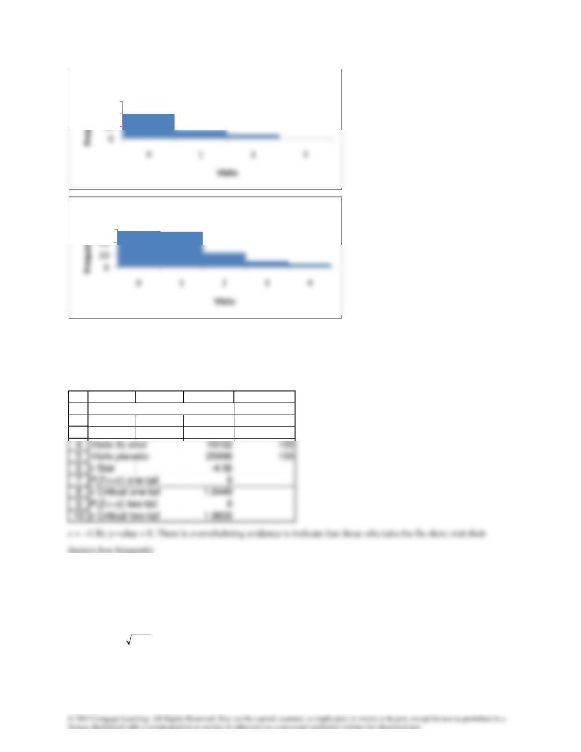
Histogram: Flu shot
60
Histogram: Placebo
The number of visits is extremely nonnormal.
Wilcoxon rank sum test
H0: The two population locations are the same
H1: The location of population 1 is to the left of the location of population 2
1
2
3
A B C D
Wilcoxon Rank Sum Test
Rank Sum Observations
A19.21 Spearman rank correlation coefficient test
a
S0 :H
= 0
S1 :H
0
1nrz S−=