18.35
15
16
19
Coefficients Standard Error t Stat P-value
18.36 All weights = .2
1
2
10
3
4
11
12
13
14
A B C D E F
SUMMARY OUTPUT
Regression Statistics
Multiple R 0.8311
df SS MS F Significance F
Regression 2 38.47 19.24 5.58 0.0532
Residual 5 17.23 3.45
Total 7 55.70
1
2
10
3
4
5
11
12
13
14
15
16
A B C D E F
SUMMARY OUTPUT
Regression Statistics
Multiple R 0.7623
R Square 0.5812
df SS MS F Significance F
Regression 2 32.37 16.19 3.47 0.1135
Residual 5 23.33 4.67
Total 7 55.70
Coefficients Standard Error t Stat P-value
19
18.37 The strength of this approach lies in regression analysis. This statistical technique allows us
18.38a
18.39a
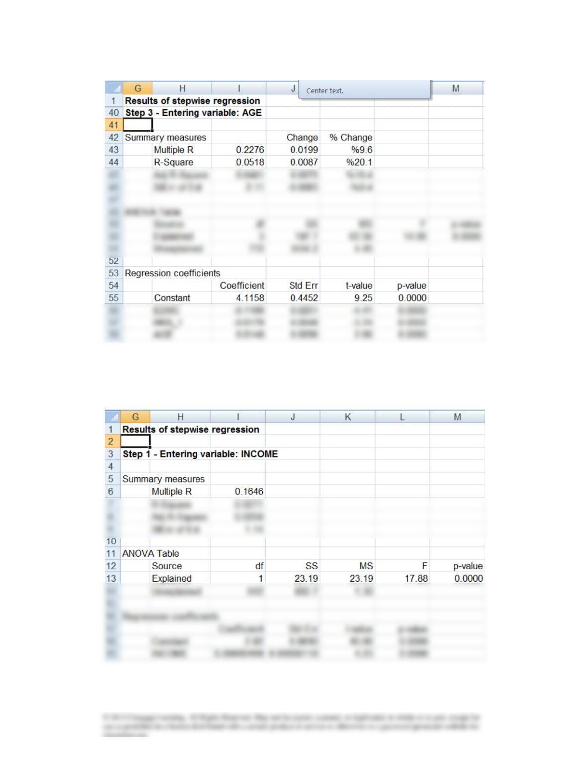
b. The only variables that were significantly linearly related to TVHOURS in Exercise 17.18 are
the only variables in the stepwise regression.
18.40
18.41
18.42
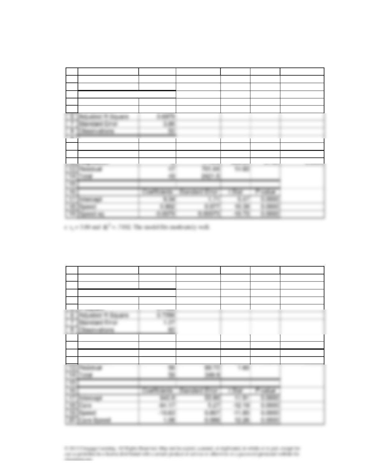
18.43a Mileage =
0
+
1
Speed +
2
Speed
2
+
b
14
15
19
18.44a Apply a first–order model with interaction.
b
14
15
1
2
3
4
5
9
10
11
A B C D E F
SUMMARY OUTPUT
Regression Statistics
Multiple R 0.8428
R Square 0.7102
ANOVA
df SS MS F Significance F
1
2
8
3
4
9
10
11
12
A B C D E F
SUMMARY OUTPUT
Regression Statistics
Multiple R 0.8623
ANOVA
df SS MS F Significance F
Regression 3 260.2 86.74 54.14 0.0000

18.45a
b F = 32.65, p-value = 0. There is enough evidence to infer that the model is valid.
18.46 a Let
1
I
= 1 if ad was in newspaper
1
I
= 0 otherwise
1
2
8
10
14
3
4
5
15
22
16
17
18
A B C D E F
SUMMARY OUTPUT
Regression Statistics
Multiple R 0.8668
R Square 0.7514
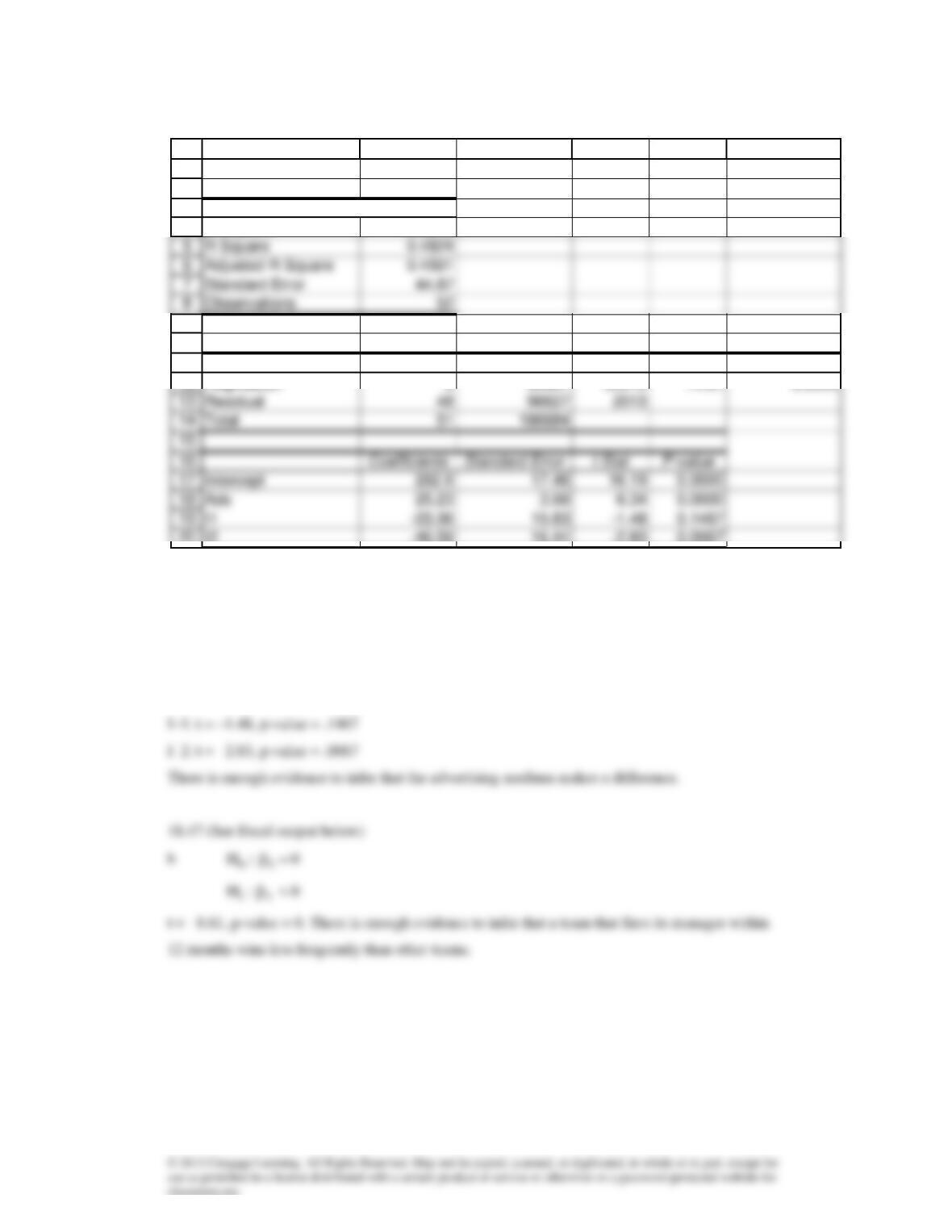
Coefficients Standard Error t Stat P-value
Intercept 404.5 327.0 1.24 0.2214
Cars -66.57 6.54 -10.19 0.0000
b
b
:H0
0
321 ===
:H1
At least on
i
is not equal to 0
F = 14.91, p-value = 0. There is enough evidence to infer that the model is valid.
c
:
0
H
=i
0
:
1
H
i
0
:H0
:H1
1
2
3
4
9
10
15
11
12
20
A B C D E F
SUMMARY OUTPUT
Regression Statistics
Multiple R 0.6946
ANOVA
df SS MS F Significance F
Regression 3 90057 30019 14.91 0.0000
I2 -46.59 16.44 -2.83 0.0067

18.48a Units =
0
+
1
Years +
2
Years
2
+
b
14
19
1
2
3
4
8
9
10
11
A B C D E F
SUMMARY OUTPUT
Regression Statistics
Multiple R 0.9347
Observations 50
ANOVA
df SS MS F Significance F
1
2
3
4
5
9
10
11
12
A B C D E F
SUMMARY OUTPUT
Regression Statistics
Multiple R 0.4351
R Square 0.1893
ANOVA
df SS MS F Significance F
Regression 2 175,291 87,646 11.32 0.0000

18.49a Depletion =
0
+
1
Temperature +
2
PH–level +
3
PH–level
2
+
44I
+
55I
+
where
1
I
= 1 if mainly cloudy
1
I
2
2
b
:H0
:H1
22
d
:H0
=1
0
:H1
1
> 0
t = 6.78, p-value = 0. There is enough evidence to infer that higher temperatures deplete chlorine
more quickly.
:H0
:H1
3
1
2
8
3
4
9
10
11
12
13
14
15
16
17
A B C D E F
SUMMARY OUTPUT
Regression Statistics
Multiple R 0.8085
ANOVA
df SS MS F Significance F
Regression 5 6596 1319 77.00 0.0000
Residual 204 3495 17.13
Total 209 10091
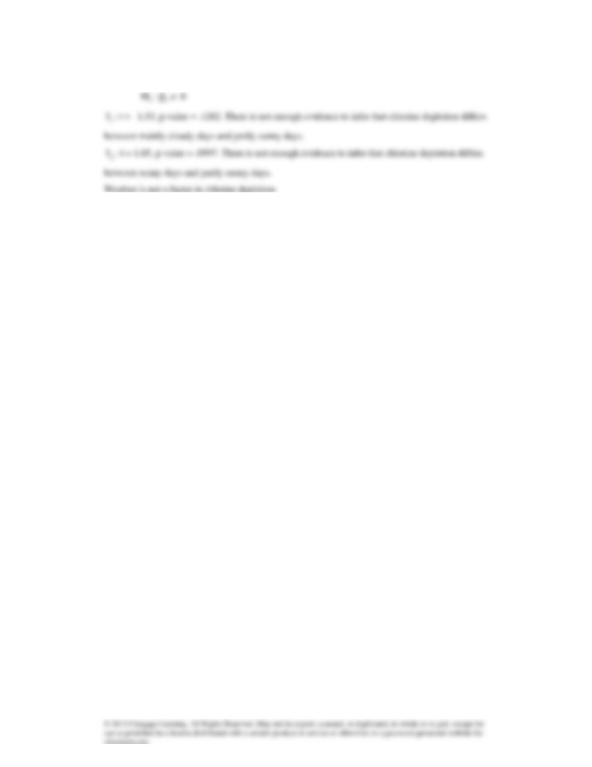
Coefficients Standard Error t Stat P-value
Intercept 1003 55.12 18.19 0.0000
f
:H0
=i
0
i