Chapter 18
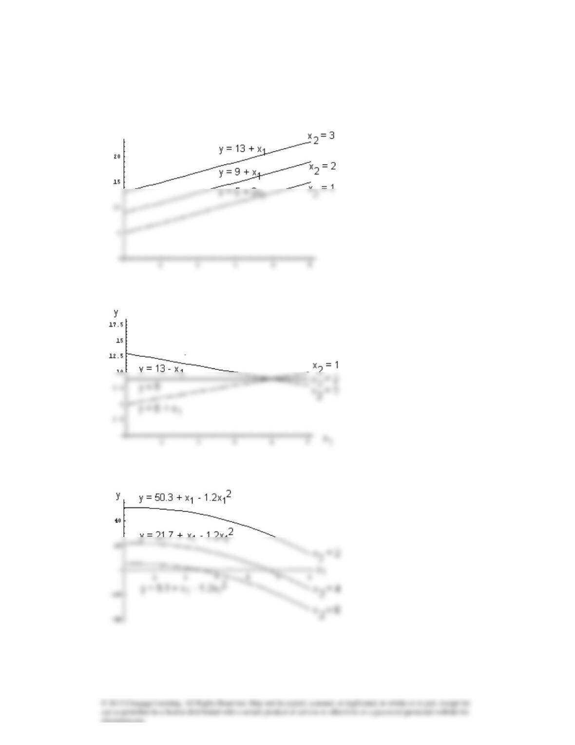
18.1 a
b
18.2 a
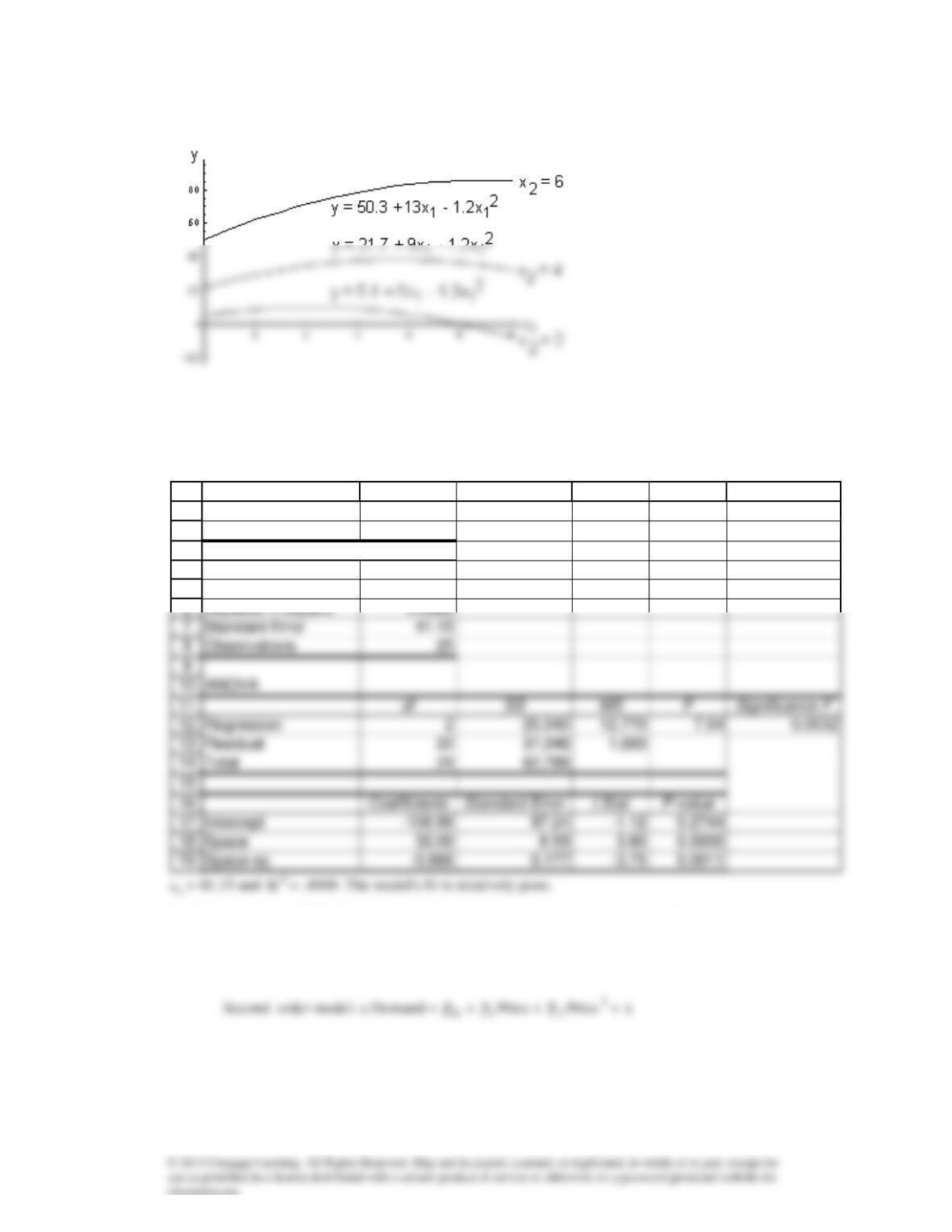
b
18.3 a Sales =
0
+
1
Space +
2
Space
2
+
b
F = 7.54, p-value = .0032. However, there is enough evidence to support the validity of the model.
18.4a First–order model: a Demand =
0
+
1
Price+
0
1
2
2
1
2
3
4
5
A B C D E F
SUMMARY OUTPUT
Regression Statistics
Multiple R 0.6378
R Square 0.4068
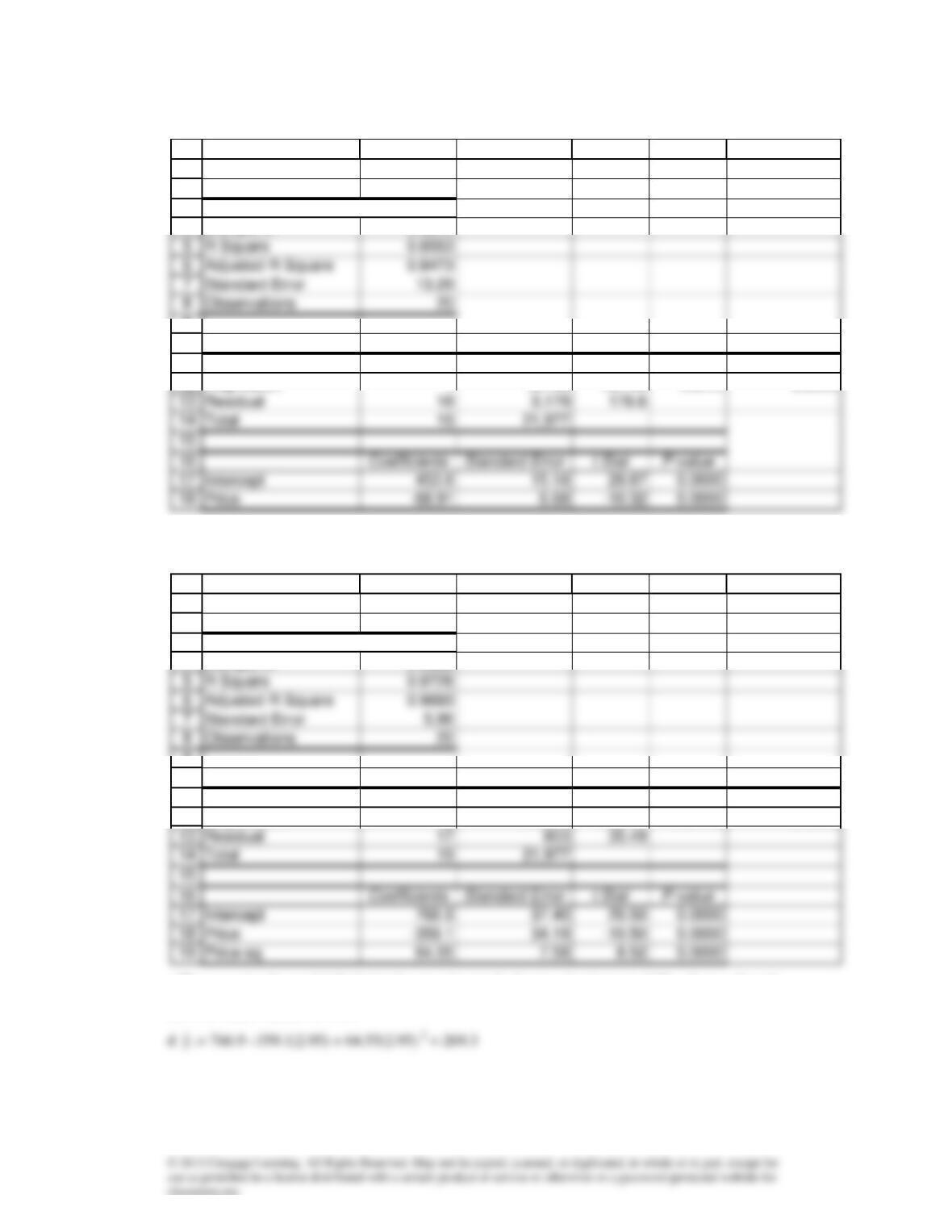
First–order model:
18
Second–order model:
14
15
19
c The second order model fits better because its standard error of estimate is 5.96, whereas that of
the first–order models is 13.29
1
2
8
3
4
9
10
11
12
A B C D E F
SUMMARY OUTPUT
Regression Statistics
Multiple R 0.9249
ANOVA
df SS MS F Significance F
Regression 1 18,798 18,798 106.44 0.0000
1
2
3
4
9
10
11
12
A B C D E F
SUMMARY OUTPUT
Regression Statistics
Multiple R 0.9862
ANOVA
df SS MS F Significance F
Regression 2 21,374 10,687 301.15 0.0000
18.5a First–order model: a Time =
0
+
1
Day+
1
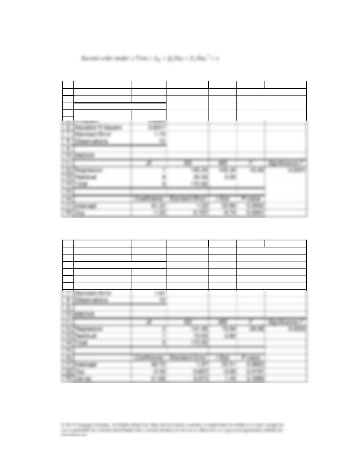
b First–order model
8
F = 45.48, p-value = 0. The model is valid.
Second–order model
F = 26.98, p-value = .0005. The model is valid.
c The second–order model is only slightly better because its standard error of estimate is smaller.
1
2
3
4
A B C D E F
SUMMARY OUTPUT
Regression Statistics
Multiple R 0.9222
1
2
3
4
5
6
A B C D E F
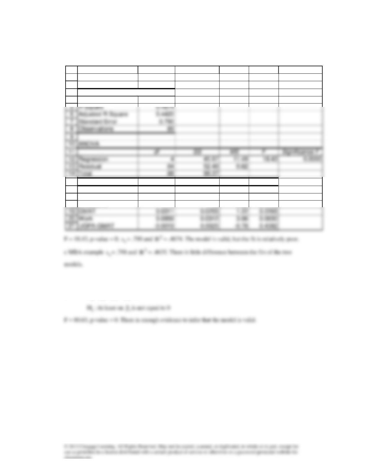
SUMMARY OUTPUT
Regression Statistics
Multiple R 0.9408
R Square 0.8852
Adjusted R Square 0.8524
18.6a MBA GPA=
0
+
1
UnderGPA +
2
GMAT +
3
Work +
4
UnderGPA
GMAT +
b
21
18.7 a (Excel output shown below)
b
:H0
0
321 ===
1
2
8
3
4
15
16
17
18
A B C D E F
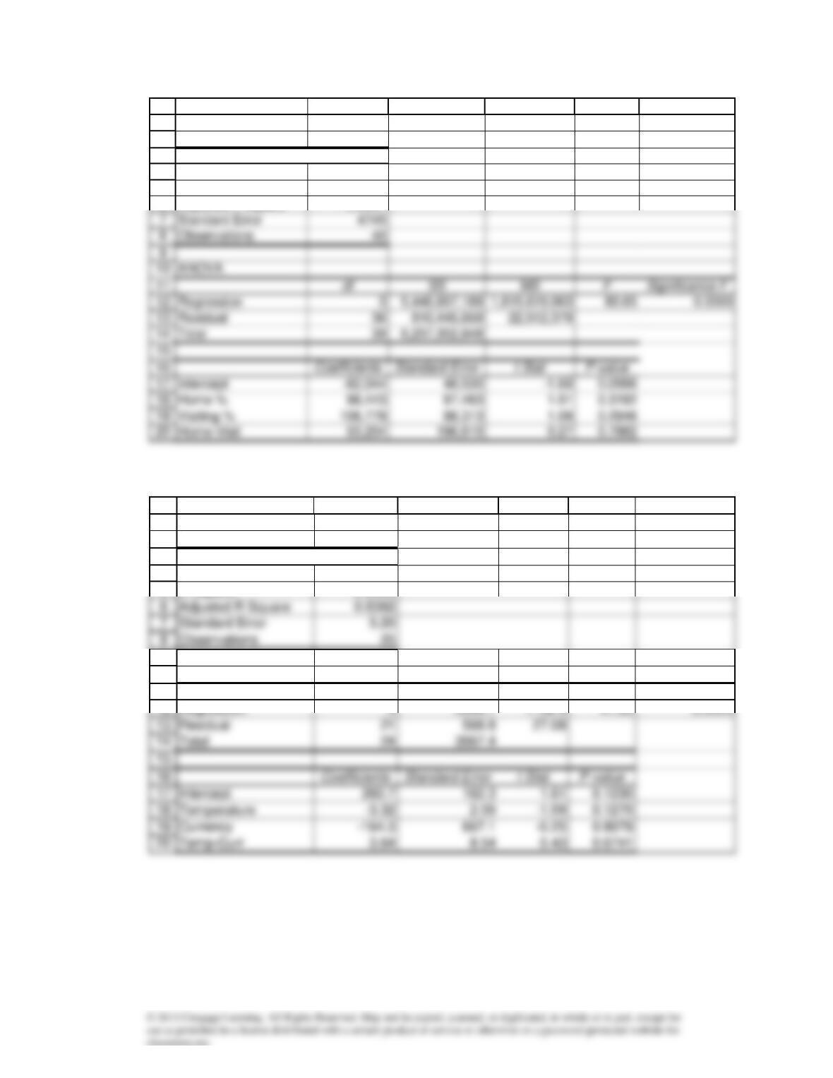
SUMMARY OUTPUT
Regression Statistics
Multiple R 0.6836
Coefficients Standard Error t Stat P-value
Intercept -11.11 14.97 -0.74 0.4601
UnderGPA 1.19 1.46 0.82 0.4159
8
18.8a
1
2
3
4
5
6
A B C D E F
SUMMARY OUTPUT
Regression Statistics
Multiple R 0.9330
R Square 0.8705
Adjusted R Square 0.8597
1
2
3
4
5
9
10
11
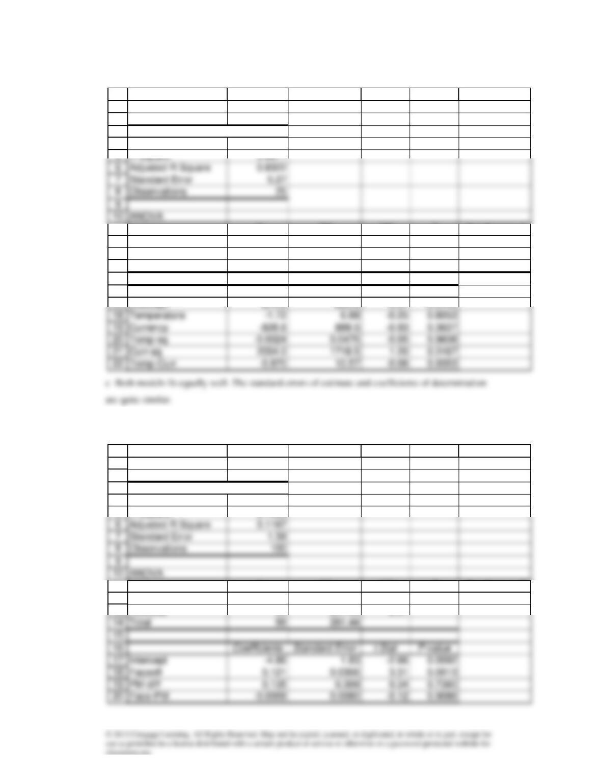
A B C D E F
SUMMARY OUTPUT
Regression Statistics
Multiple R 0.9255
R Square 0.8566
ANOVA
df SS MS F Significance F
b
22
18.9a
1
2
8
10
3
4
11
12
13
14
15
16
17
A B C D E F
SUMMARY OUTPUT
Regression Statistics
Multiple R 0.9312
df SS MS F Significance F
Regression 5 3440.3 688.1 24.80 0.0000
Residual 19 527.1 27.74
Total 24 3967.4
Coefficients Standard Error t Stat P-value
Intercept 274.8 283.8 0.97 0.3449
1
2
8
3
4
5
11
12
13
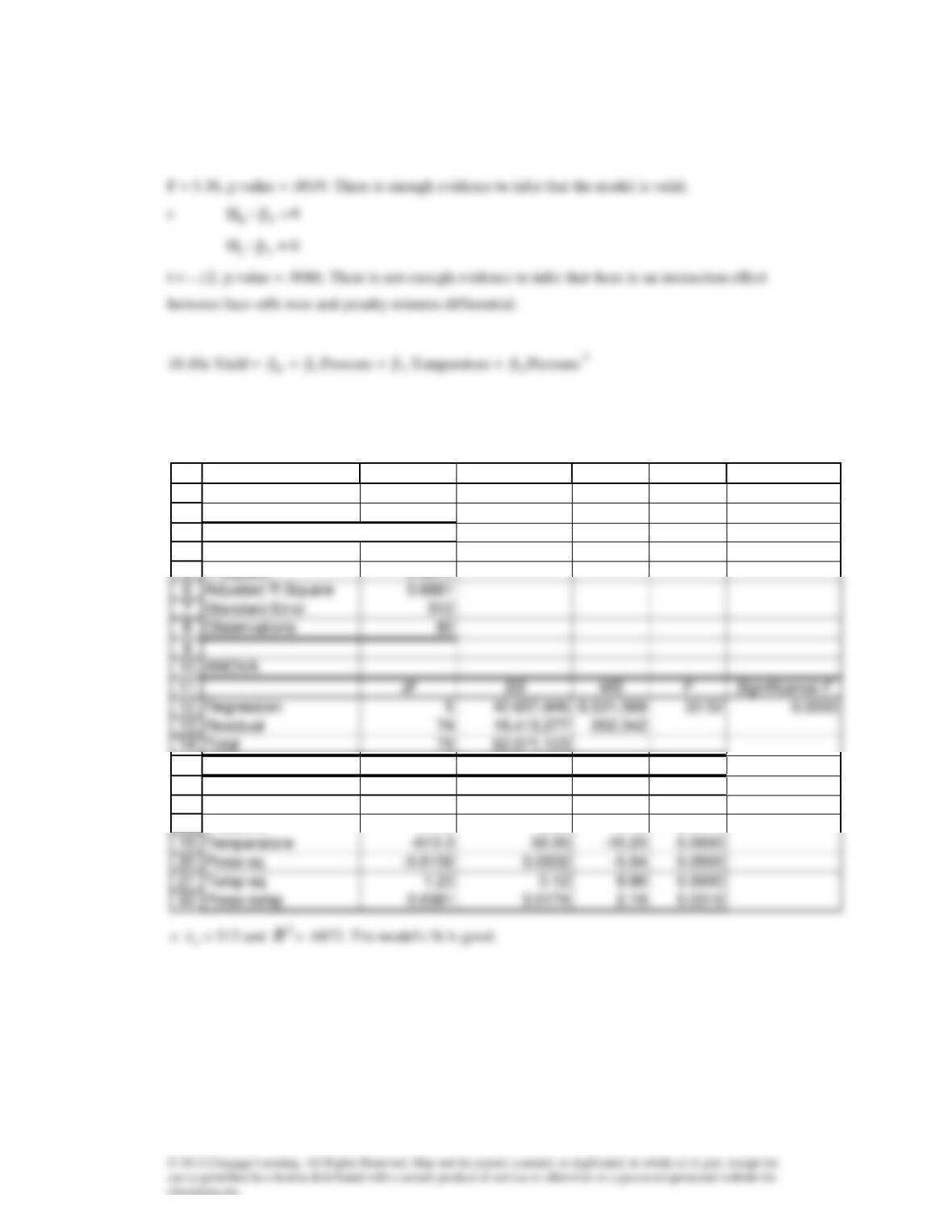
A B C D E F
SUMMARY OUTPUT
Regression Statistics
Multiple R 0.3788
R Square 0.1435
df SS MS F Significance F
Regression 3 40.38 13.46 5.36 0.0019
Residual 96 241.06 2.51
b
:H0
0
321 ===
:H1
At least on
i
is not equal to 0
:H0
:H1
3
3
2
+
4
Temperature
2
+
5
Pressure Temperature +
b
22
18.11 The number of indicator variables is m – 1 = 5 – 1 = 4.
1
2
8
10
14
3
4
5
15
16
17
18
A B C D E F
SUMMARY OUTPUT
Regression Statistics
Multiple R 0.8290
R Square 0.6872
Coefficients Standard Error t Stat P-value
Intercept 74462 7526 9.89 0.0000
Pressure 14.40 5.92 2.43 0.0174
18.12 a
1
I
= 1 if Catholic
1
I
= 0 otherwise
1
I
1
I
c
1
I
= 1 if Jack Jones
1
I
= 0 otherwise
18.13 a Macintosh b IBM c other
18.14
=
1
I
1 if B.A.
= 0 otherwise
I
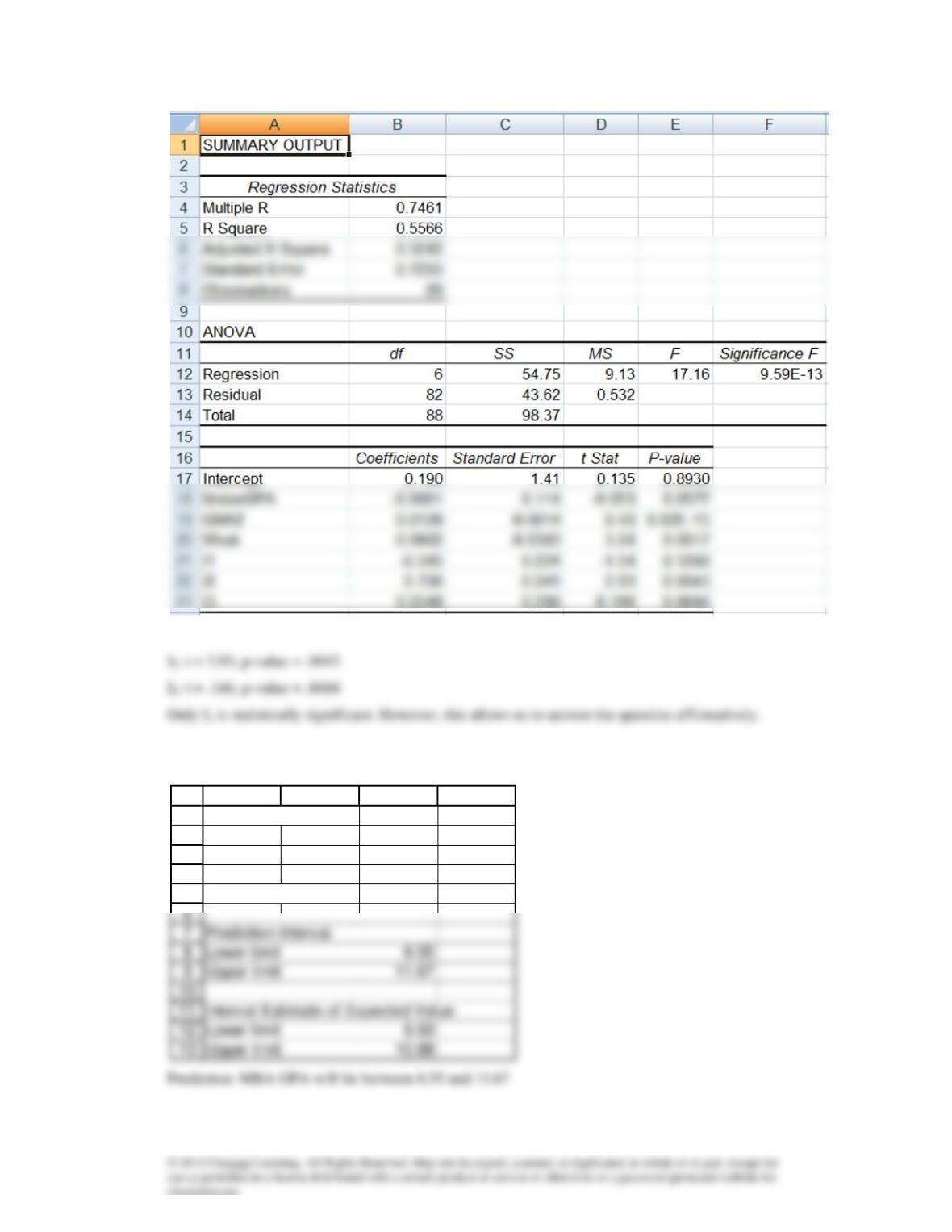
I1: t = -1.54, p-value = .1269
18.15a
1
2
3
4
5
A B C D
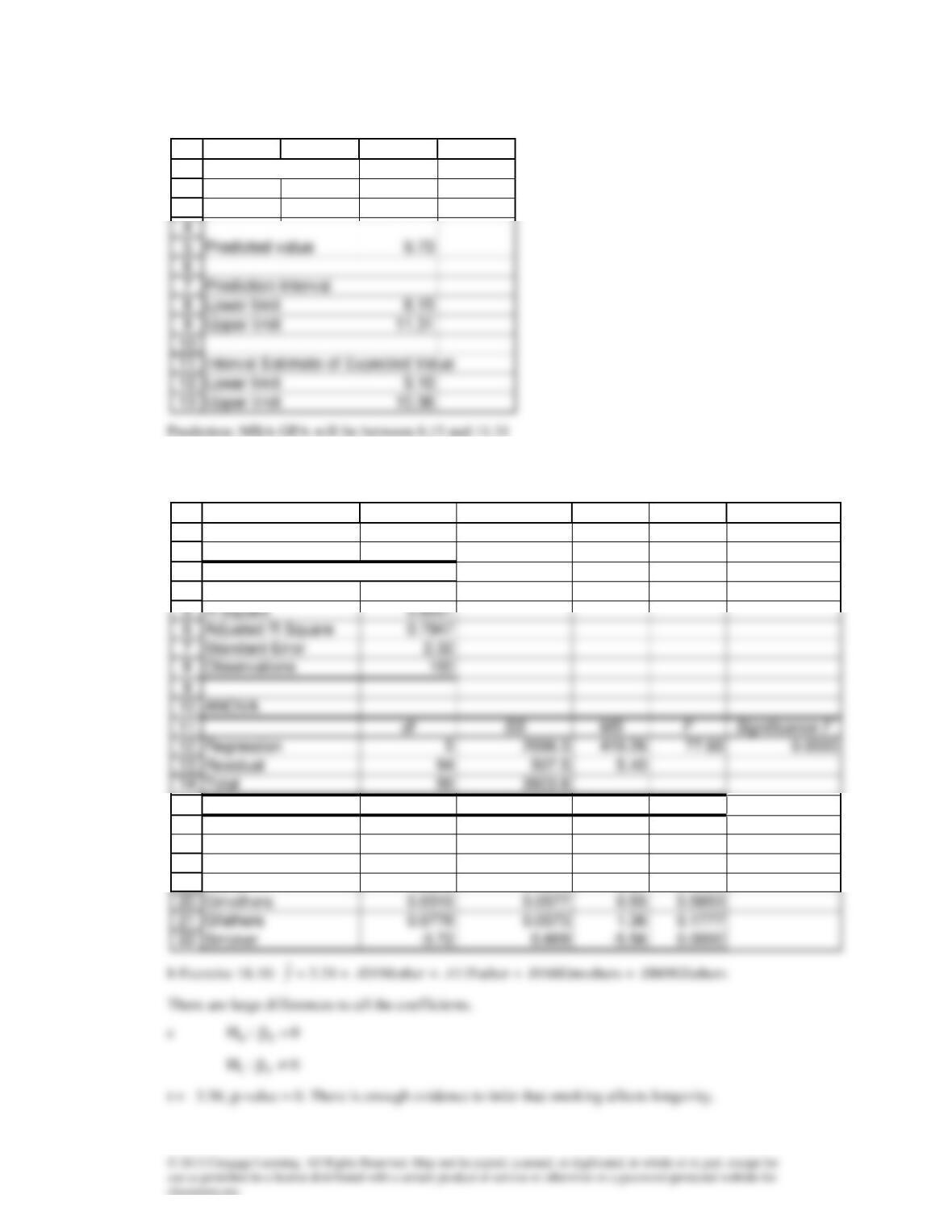
Prediction Interval
MBA GPA
Predicted value 10.11
b
18.16a
22
1
2
3
A B C D
Prediction Interval
MBA GPA
1
2
8
10
14
3
4
15
16
17
18
19
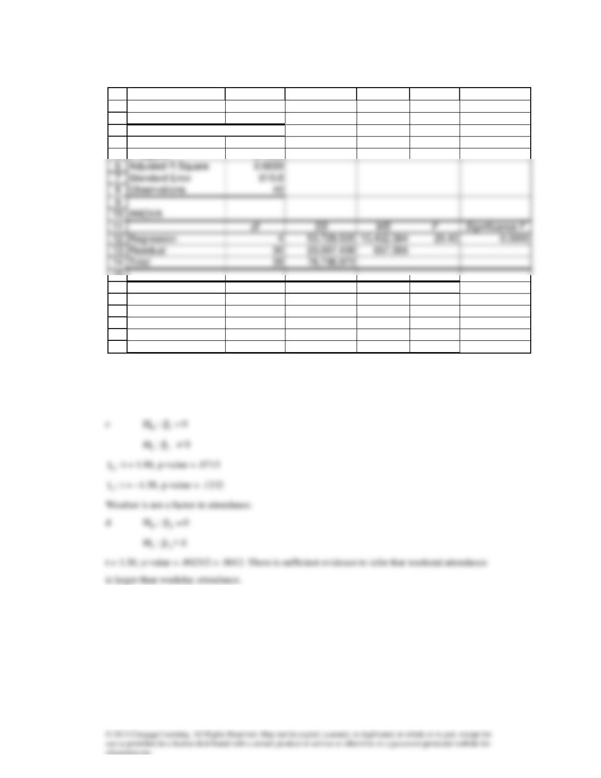
A B C D E F
SUMMARY OUTPUT
Regression Statistics
Multiple R 0.8973
Coefficients Standard Error t Stat P-value
Intercept 23.57 5.98 3.94 0.0002
Mother 0.306 0.0542 5.65 0.0000
Father 0.303 0.0476 6.37 0.0000
18.17a
b
:H0
0
4321 ====
:H1
At least on
i
is not equal to 0
F = 20.43, p-value = 0. There is enough evidence to infer that the model is valid.
:H0
:H1
:H0
:H1
1
2
10
14
3
4
5
15
16
17
18
19
20
21
A B C D E F
SUMMARY OUTPUT
Regression Statistics
Multiple R 0.8368
R Square 0.7002
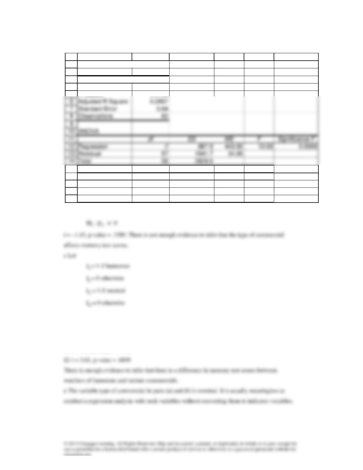
Coefficients Standard Error t Stat P-value
Intercept 3490 469.2 7.44 0.0000
Yest Att 0.369 0.078 4.73 0.0000
I1 1623 492.5 3.30 0.0023
I2 733.5 394.4 1.86 0.0713
I3 -765.5 484.7 -1.58 0.1232
18.18a
b
:H0
=2
0
:H1
See Excel output below.
d
:H0
=i
0
:H1
i
0
I1: t = 1.61, p-value = .1130
1
2
8
3
4
15
16
17
18
19
A B C D E F
SUMMARY OUTPUT
Regression Statistics
Multiple R 0.5602
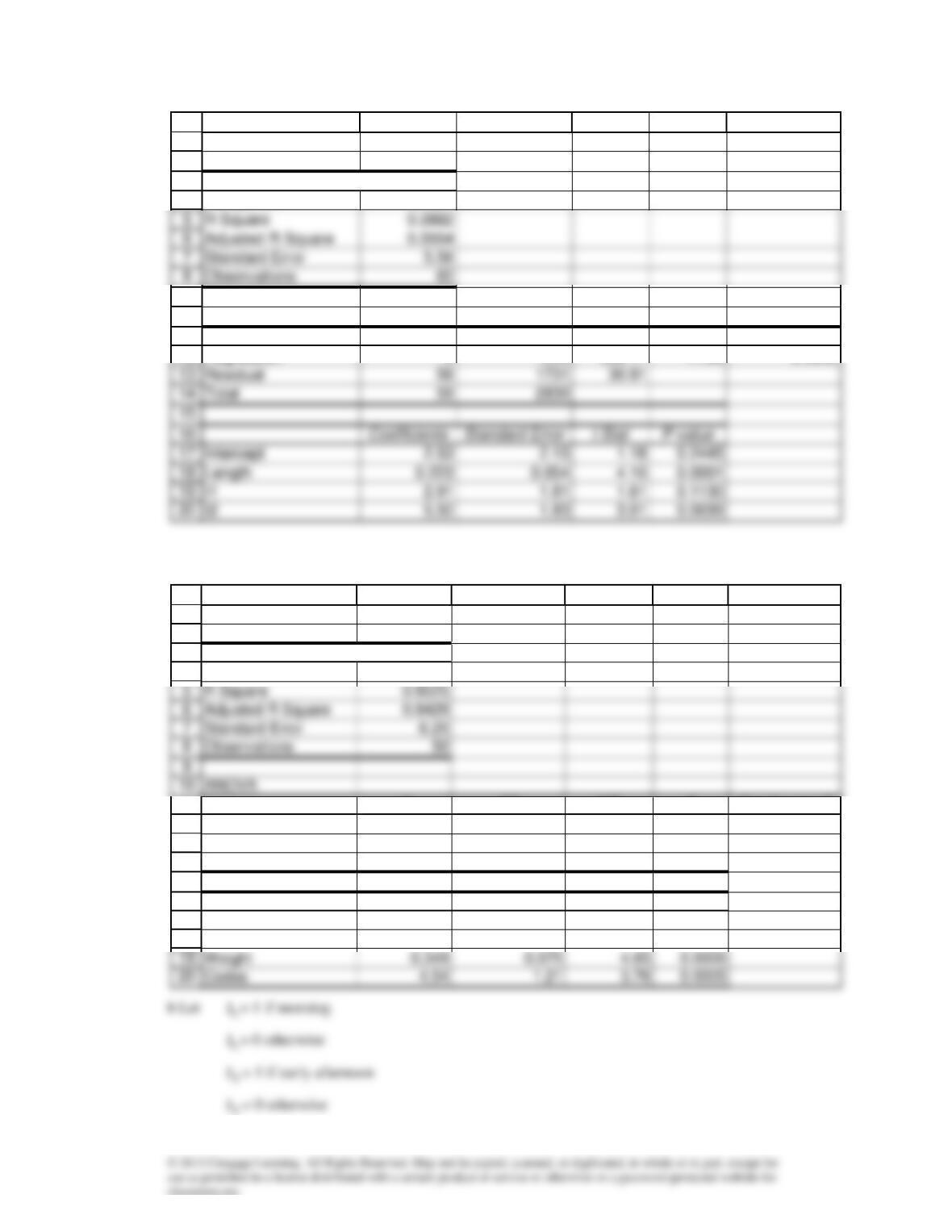
Coefficients Standard Error t Stat P-value
Intercept 7.02 3.24 2.17 0.0344
Length 0.250 0.056 4.46 0.0000
Type -1.35 0.947 -1.43 0.1589
15
20
18.19 a
1
2
3
4
9
10
11
12
A B C D E F
SUMMARY OUTPUT
Regression Statistics
Multiple R 0.6231
ANOVA
df SS MS F Significance F
Regression 3 1099 366.17 11.85 0.0000
1
2
8
10
3
4
11
12
13
14
15
16
17
18
A B C D E F
SUMMARY OUTPUT
Regression Statistics
Multiple R 0.9233
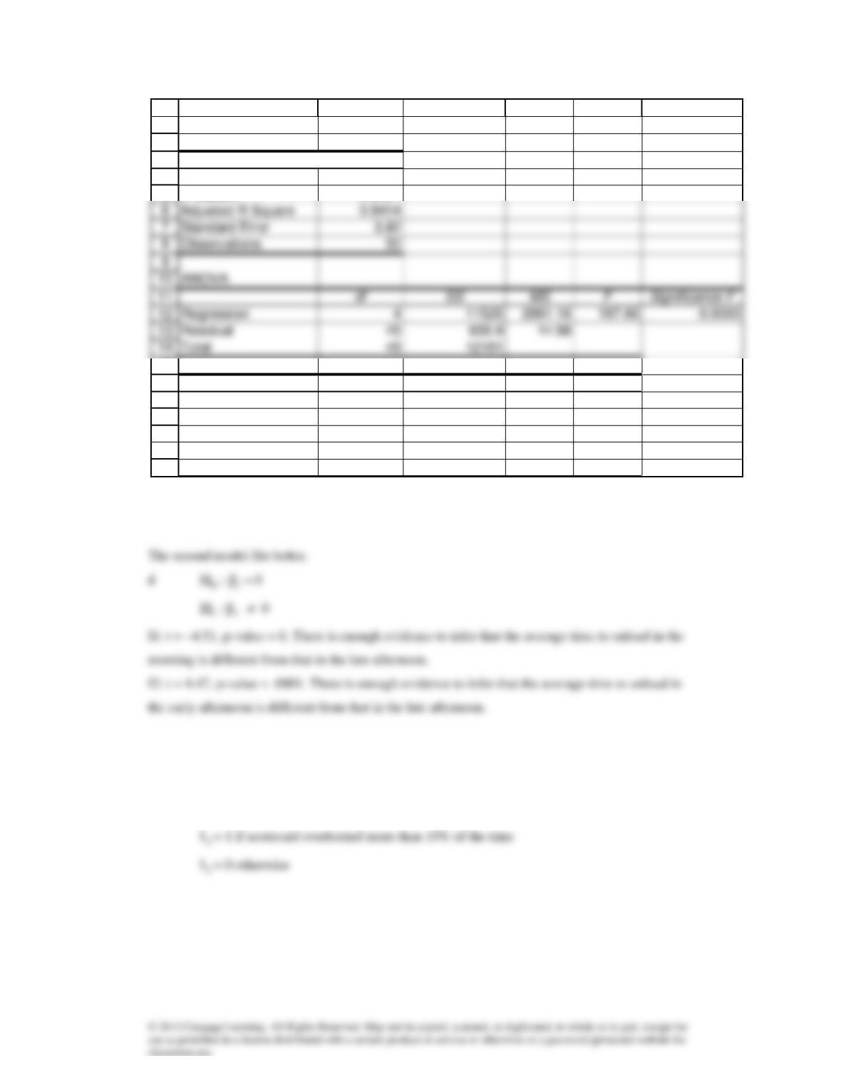
df SS MS F Significance F
Regression 3 10384 3461.40 88.64 0.0000
Residual 46 1796 39.05
Total 49 12181
Coefficients Standard Error t Stat P-value
Intercept -41.42 7.00 -5.92 0.0000
Boxes 0.644 0.050 12.79 0.0000
c Model 1:
s
= 6.25 and
2
R
= .8525.
Model 2:
s
= 3.82 and
2
R
= .9461.
18.20a Let
1
I
= 1 if no scorecard
1
I
= 0 otherwise
1
2
8
3
4
5
15
16
17
18
19
20
21
A B C D E F
SUMMARY OUTPUT
Regression Statistics
Multiple R 0.9727
R Square 0.9461
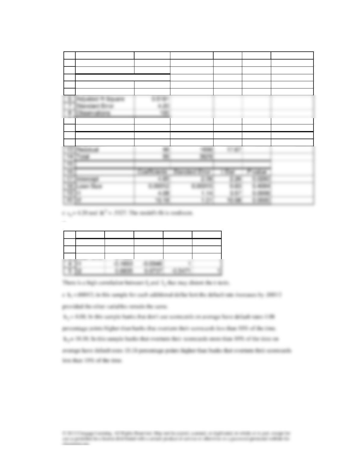
Coefficients Standard Error t Stat P-value
Intercept -29.72 3.73 -7.97 0.0000
Boxes 0.618 0.031 19.99 0.0000
Weight 0.346 0.046 7.54 0.0000
I1 -6.76 1.50 -4.51 0.0000
I2 6.48 1.45 4.47 0.0001
b
15
20
d
1
2
3
4
5
9
10
11
12
A B C D E F
SUMMARY OUTPUT
Regression Statistics
Multiple R 0.7299
R Square 0.5327
ANOVA
df SS MS F Significance F
Regression 3 1933 644.46 36.48 0.0000
1
2
3
A B C D E
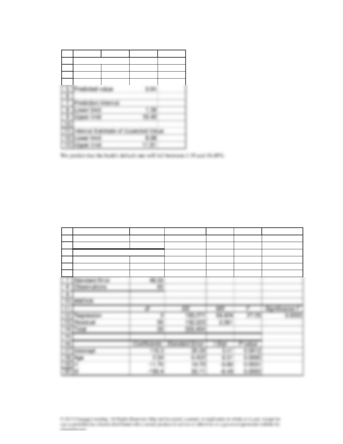
Pct Bad Loan Size I1 I2
Pct Bad 1
Loan Size 0.1099 1
f
18.21 a Let
1
I
= 1 if welding machine
1
I
= 0 otherwise
2
I
= 1 if lathe
2
I
= 0 otherwise
1
2
3
4
A B C D
Prediction Interval
Pct Bad
1
2
3
4
5
6
A B C D E F
SUMMARY OUTPUT
Regression Statistics
Multiple R 0.7706
R Square 0.5938
Adjusted R Square 0.5720
b
1
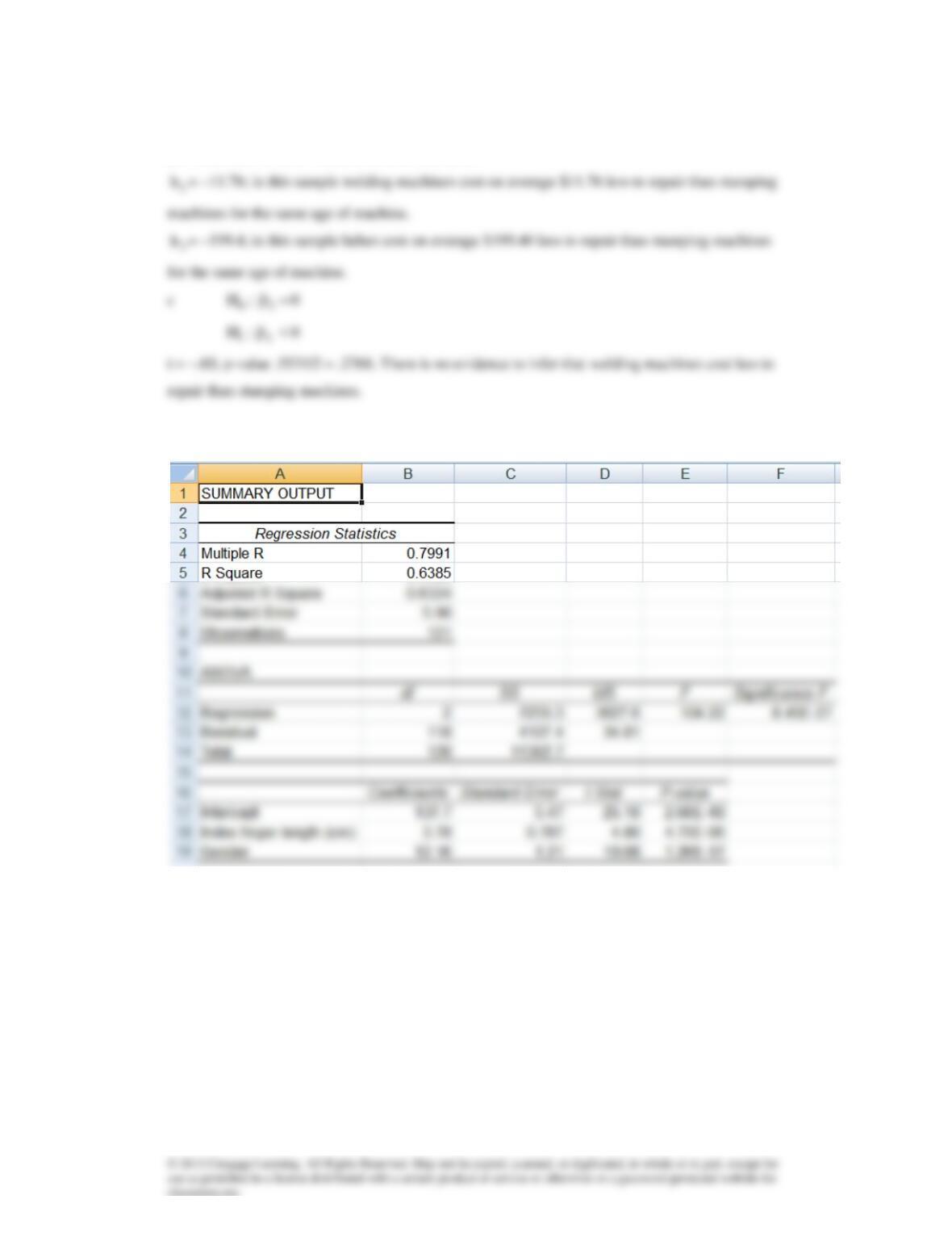
b
= 2.54; in this sample for each additional month repair costs increase on average by $2.54
provided that the other variable remains constant.
18.22
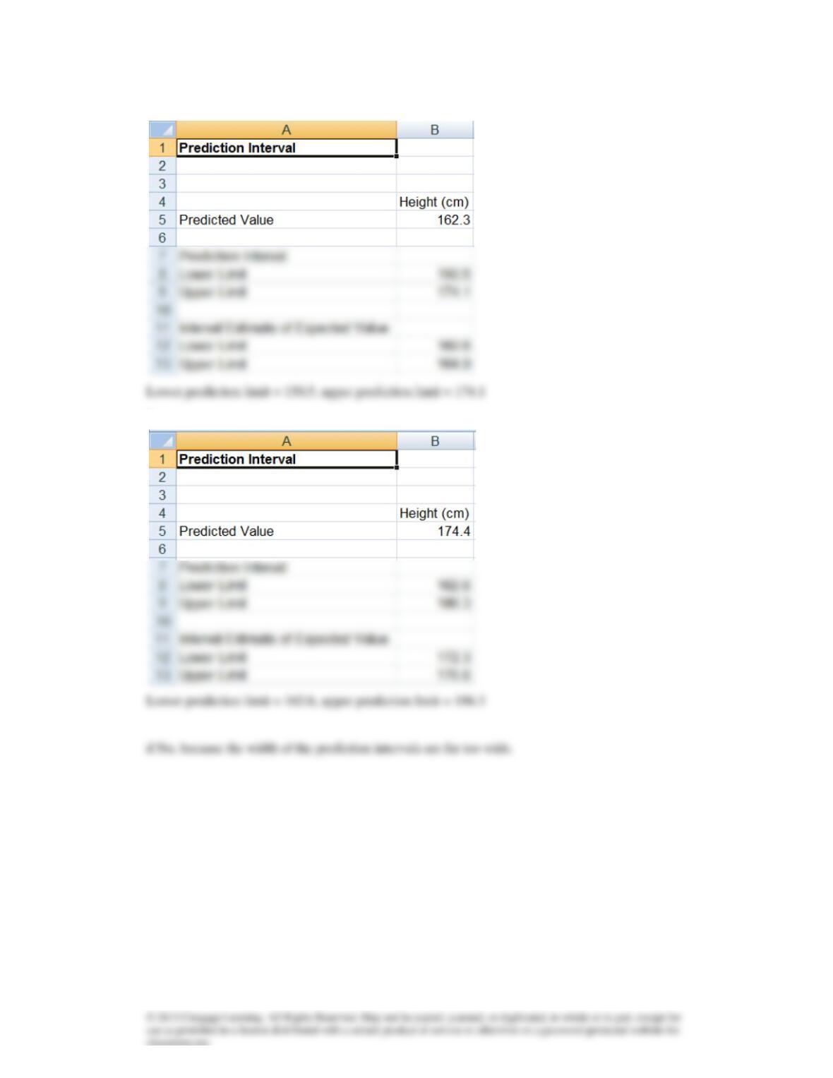
a. The coefficient of determination in Exercise 16.107 was .3270. In this model the coefficient of
determination is .6385. This model is better.
b
c
18.23a
4
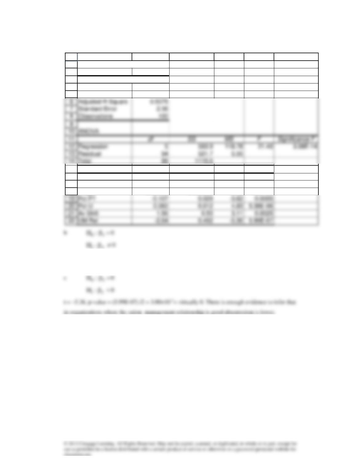
t = 3.11, p-value = .0025. There is enough evidence to infer that the availability of shiftwork
affects absenteeism.
5
1
2
8
10
14
3
4
5
15
16
17
18
A B C D E F
SUMMARY OUTPUT
Regression Statistics
Multiple R 0.7296
R Square 0.5323
Coefficients Standard Error t Stat P-value
Intercept 10.26 1.17 8.76 8.12E-14
Wage -0.00020 0.000036 -5.69 1.43E-07