│ REAL STATISTICS–REAL DECISIONS 535
CHAPTER 1
REAL STATISTICS–REAL DECISIONS
1. (a) Answers will vary.
(b) Yes
2. (a) Both, because questions will ask for demographics (qualitative) as well as cost (quantitative)
(b) Gender, business/recreational: Nominal
Cost of ticket: Ratio
Comfort, safety: Ordinal
CHAPTER 2
REAL STATISTICS–REAL DECISIONS
1. (a) Find the average cost of renting an apartment for each area and do a comparison.
(b) The mean would best represent the data sets for the four areas of the city.
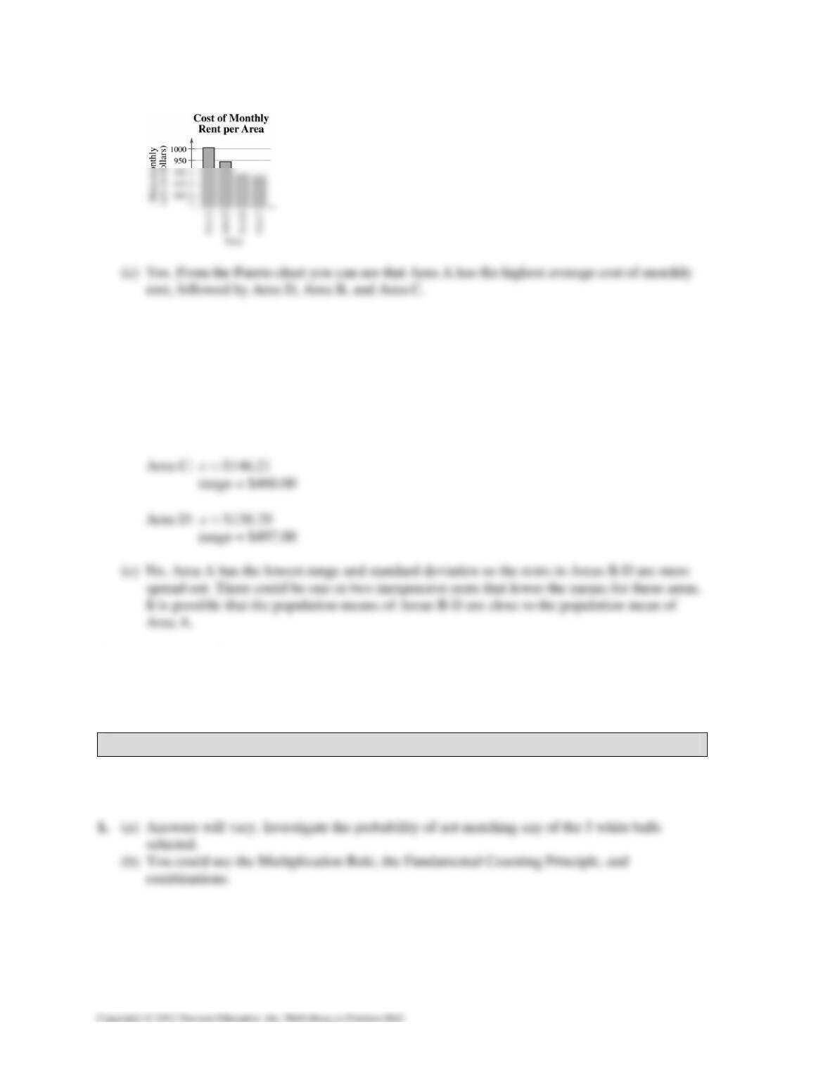
2. (a) Construct a Pareto chart, because the data are quantitative and a Pareto chart positions data in
order of decreasing height, with the tallest bar positioned at the left.
536 REAL STATISTICS–REAL DECISIONS │
(b)
3. (a) You could use the range and sample standard deviation for each area.
(b) Area A: $123.07s≈
range = $415.00
Area B: $144.91s≈
range = $421.00
4. (a) Answers will vary.
(b) Location, weather, population
CHAPTER 3
REAL STATISTICS–REAL DECISIONS
│ REAL STATISTICS–REAL DECISIONS 537
2. If you played only the red ball, the probability of matching it is 1
39 . However, because you must
pick five white balls, you must get the white balls wrong. So, using the Multiplication Rule, you
get
3. The overall probability of winning a prize is determined by calculating the number of ways to win
and dividing by the total number of outcomes.
To calculate the number of ways to win something, you must use combinations.
CHAPTER 4
REAL STATISTICS–REAL DECISIONS
1. (a) Answers will vary. For instance, calculate the probability of obtaining 0 clinical pregnancies
out of 10 randomly selected ART cyclos.
(b) Binomial. The distribution is discrete because the number of clinical pregnancies is
countable.
2. n = 10, p = 0.349, P(0) = 0.014
x P(x)
0 0.01367
1 0.07329
2 0.17681
3 0.25277
3. (a) Suspicious, because the probability is very small.
(b) Not suspicious, because the probability is not that small.
538 REAL STATISTICS–REAL DECISIONS │
CHAPTER 5
REAL STATISTICS–REAL DECISIONS
1. 60, 0.75
45 5, 15 5
np
np nq
==
=≥ =≥
Can use normal distribution.
2. (a) 56 0.67
1.5
x
zµ
σ
−−
==≈−
( 5) ( 0.67) 0.2514Px Pz<= <− =
(b) 56 0.67
1.5
x
zµ
σ
−−
==≈−
CHAPTER 6
REAL STATISTICS–REAL DECISIONS
1. (a) Yes, there has been a change in the mean concentration level because the confidence interval
for Year 1 does not overlap the confidence interval for Year 2.
│ REAL STATISTICS–REAL DECISIONS 539
3. The width of the confidence interval for Year 2 may have been caused by greater variation in the
levels of cyanide than in other years, which may be the result of outliers.
CHAPTER 7
REAL STATISTICS–REAL DECISIONS
1. (a)-(c) Answers will vary.
2. 0: 0.50; : 0.50 (claim)
a
Hp Hp≤>
l
280 0.5
560
x
pn
== =
CHAPTER 8
REAL STATISTICS–REAL DECISIONS
1. (a) Answers will vary. Sample answer: Divide the records into groups according to the
inpatients’ ages, and then randomly select records from each group.
540 REAL STATISTICS–REAL DECISIONS │
2. (a) Answers will vary.
(b) Answers will vary.
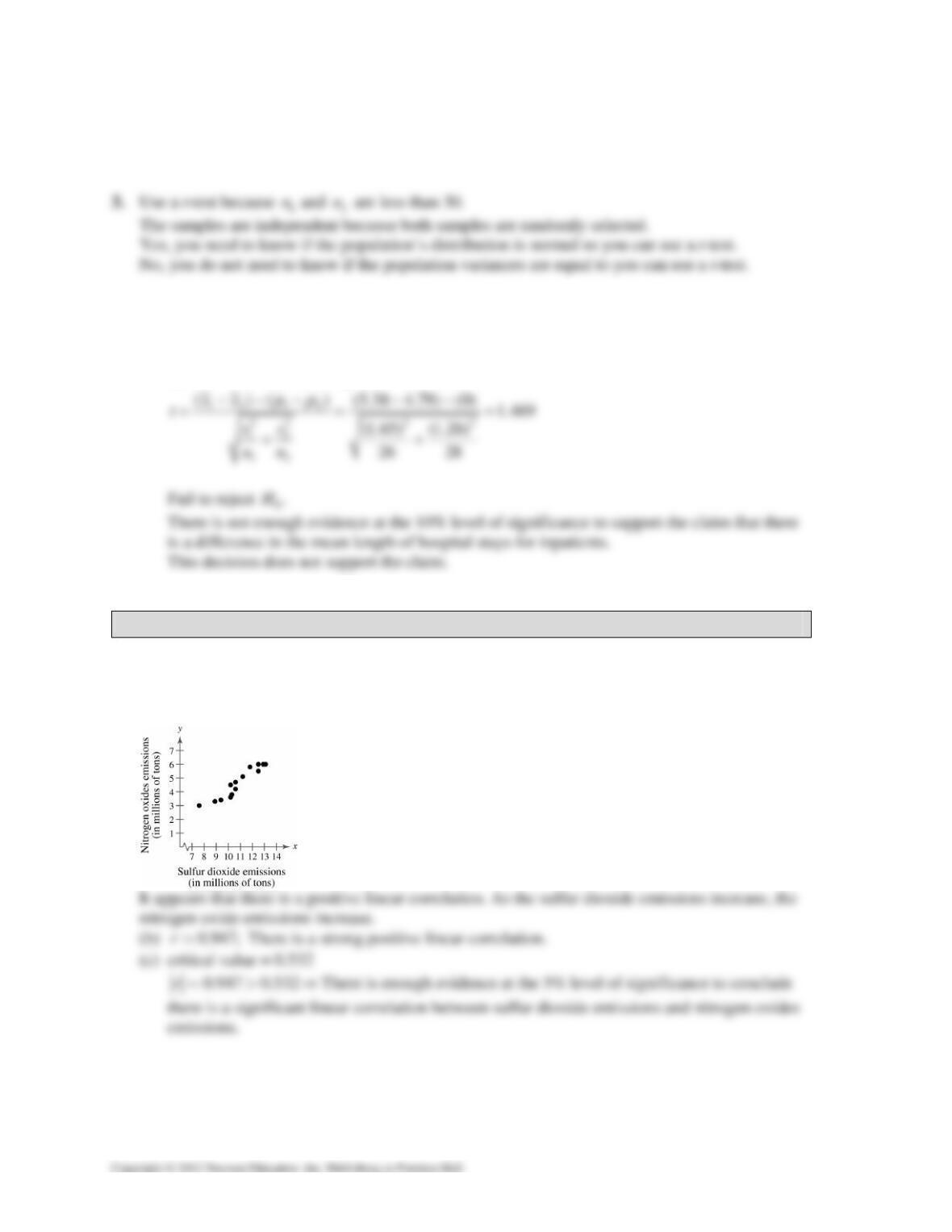
4. The claim is “there is a difference in the mean length of hospital stays for inpatients.”
01 2 1 2
:; : (claim)
a
HH
µ
µµµ
=≠
d.f. = 12
min{ 1, 1} 25nn−−=
01.708;t=± Rejection region: 1.708, 1.708tt<− >
CHAPTER 9
REAL STATISTICS–REAL DECISIONS
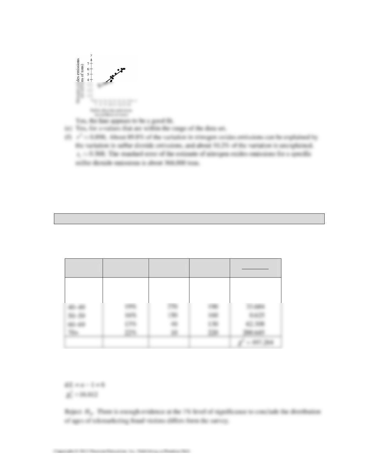
1. (a)
│ REAL STATISTICS–REAL DECISIONS 541
(d)
0.652 2.438yx=−
2. 1.358 3.286y<<
You can be 95% confident that the nitrogen oxides emissions will be between 1.358 and 3.286
million tons when the sulfur dioxide emissions are 17.3 – 10 = 7.3 million tons.
CHAPTER 10
REAL STATISTICS–REAL DECISIONS
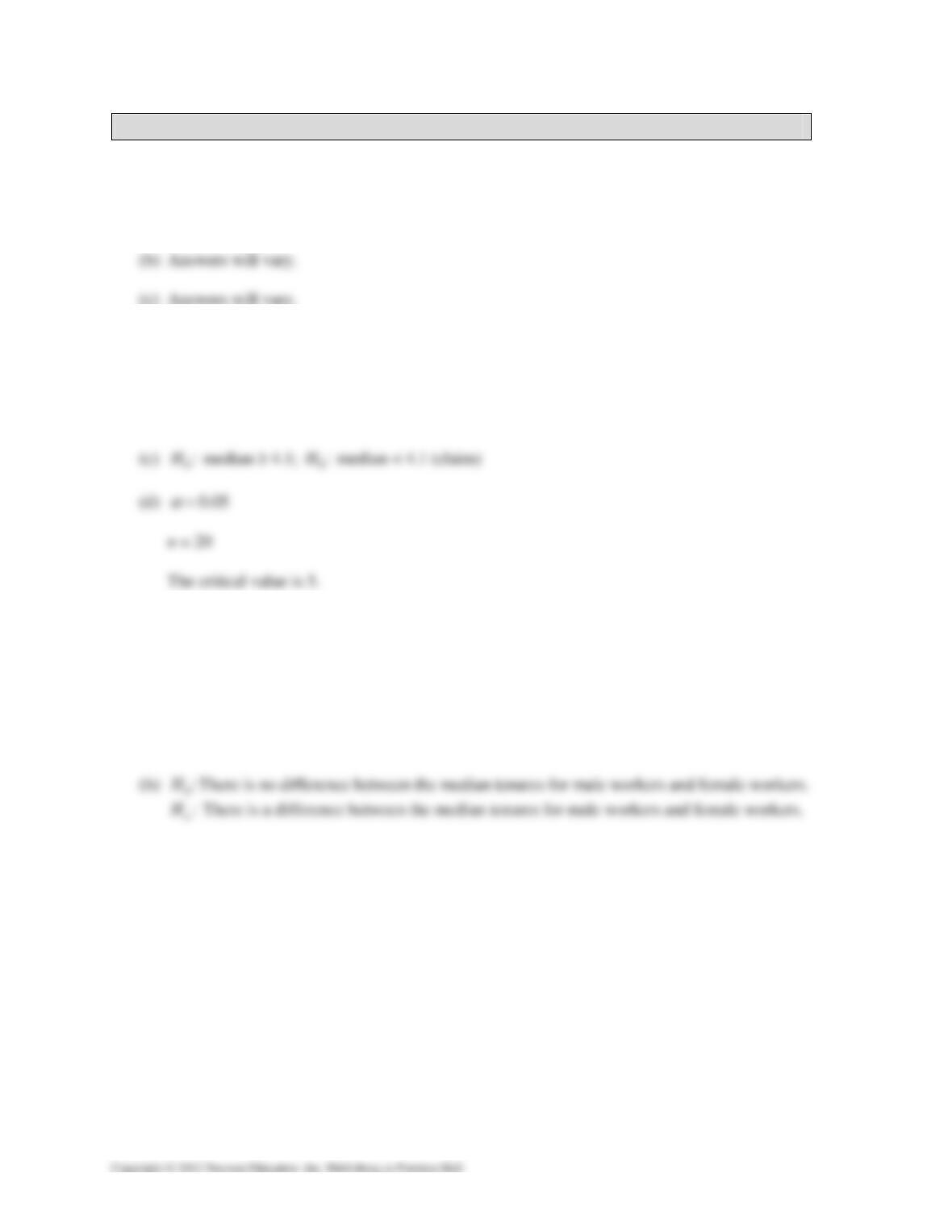
1.
Age Distribution Observed Expected OE
E
2
()−
Under 20 1% 30 10 40.000
20−39 13% 200 130 37.692
30−39 16% 300 160 122.500
0:HThe distribution of ages is as shown in the table above. (claim)
:
a
H The distribution of ages differs from the claimed distribution.
542 REAL STATISTICS–REAL DECISIONS │
CHAPTER 11
REAL STATISTICS–REAL DECISIONS
1. (a) Answers will vary.
2. (a) Answers will vary. For example, ask “Is the data a random sample?” and “Is the data
normally distributed?”
(b) Sign test; You need to use the nonparametric test because nothing is known about the shape
of the population.
x = 7
Fail to reject
0.H There is not enough evidence at the 5% level of significance to support the
claim that the median tenure is less than 4.1 years.
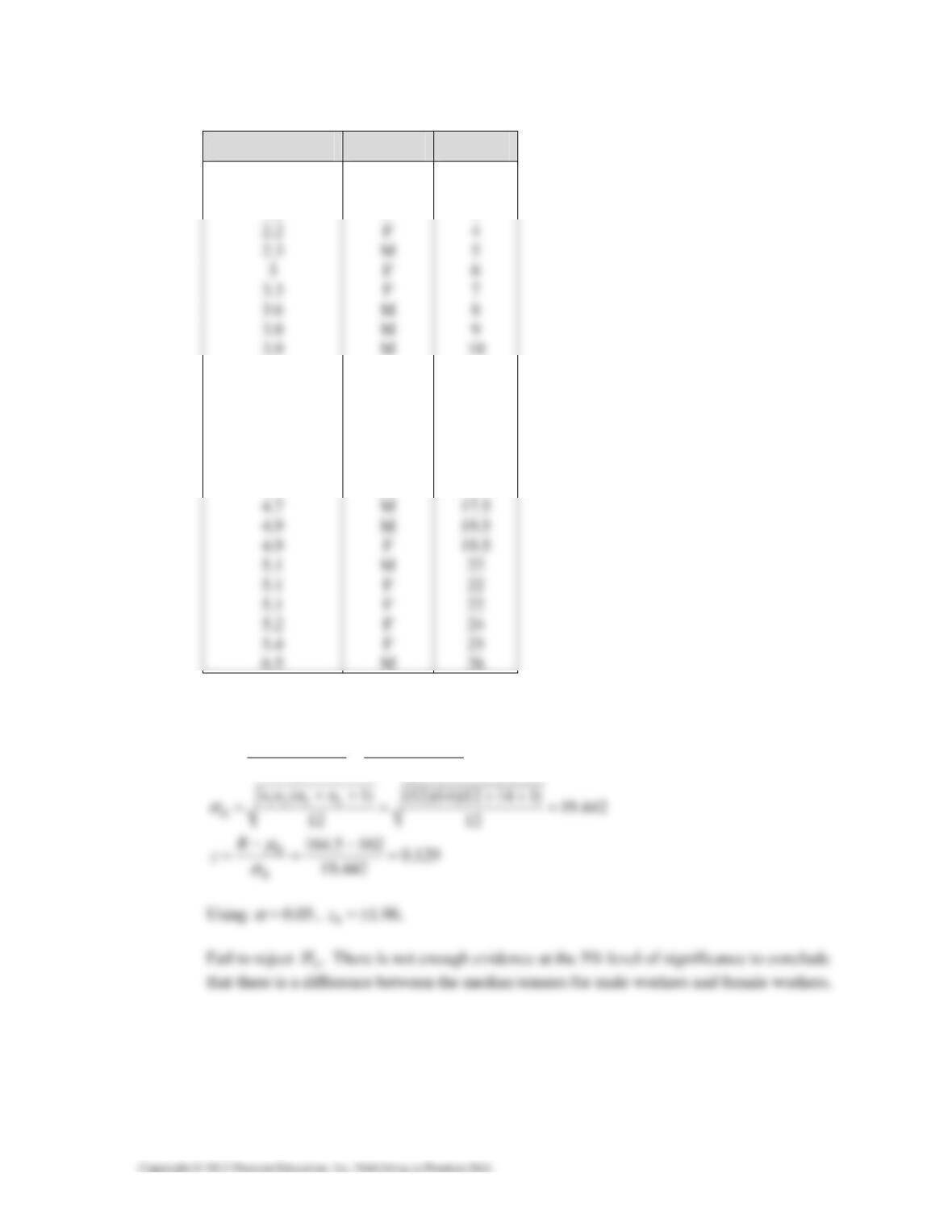
3. (a) Because the data from each sample appears non-normal, the Wilcoxon rank sum test should
be used.
│ REAL STATISTICS–REAL DECISIONS 543
(c)
Ordered data Sample Rank
0.9 M 1
1.3 F 2
1.8 F 3
4 F 11.5
4 F 11.5
4.3 M 13.5
4.3 F 13.5
4.4 M 15.5
4.4 F 15.5
4.7 M 17.5
R = sum ranks of male workers = 164.5
11 2
(1)
12(12141) 162
22
R
nn n
µ
++ ++
===