Solution 18.1
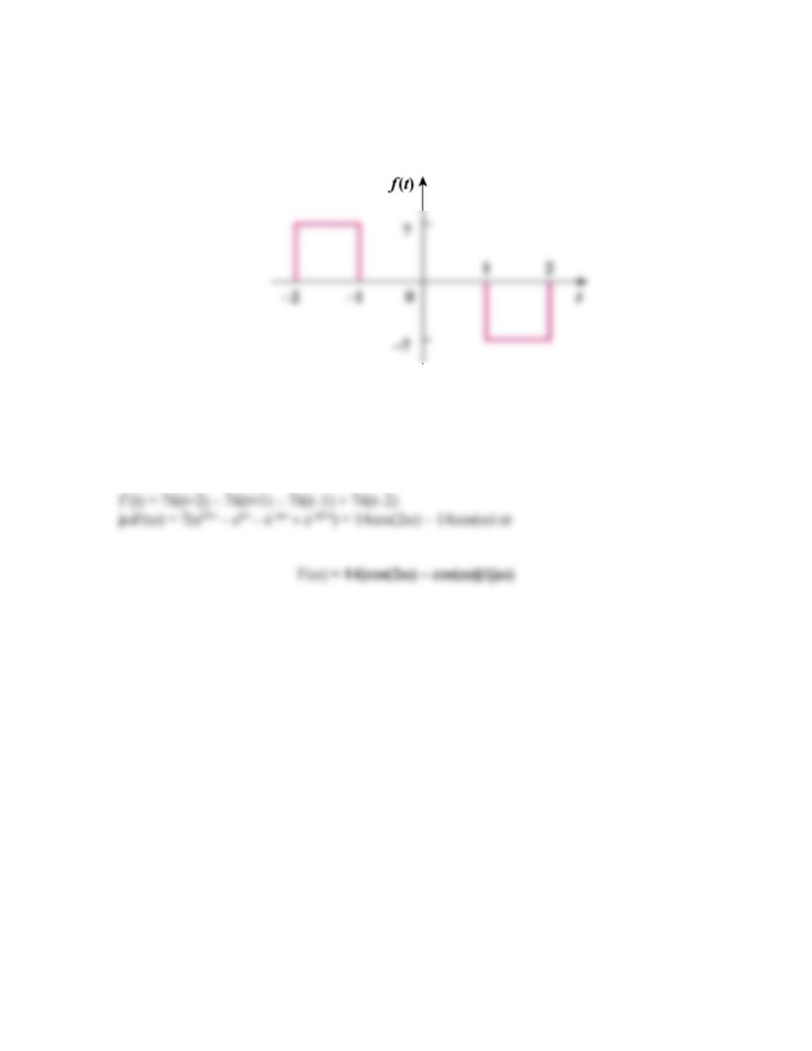
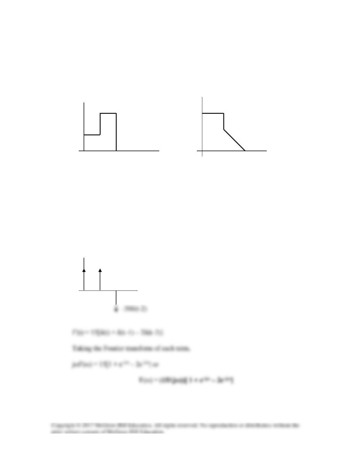
Obtain the Fourier transform of the function in Fig. 18.26.
Figure 18.26
For Prob. 18.1.
Solution
f(t) = 7u(t+2) – 7u(t+1) – 7u(t–1) + 7u(t–2)
Solution 18.2
Using Fig. 18.27, design a problem to help other students to better understand the Fourier
transform given a wave shape.
Although there are many ways to solve this problem, this is an example based on the same kind
of problem asked in the third edition.
Problem
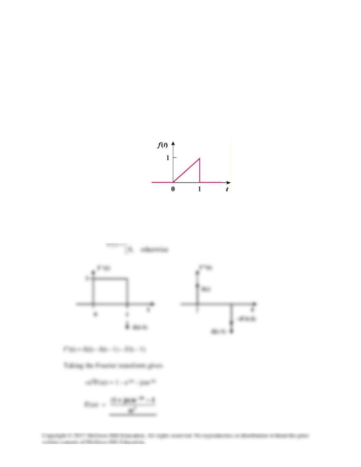
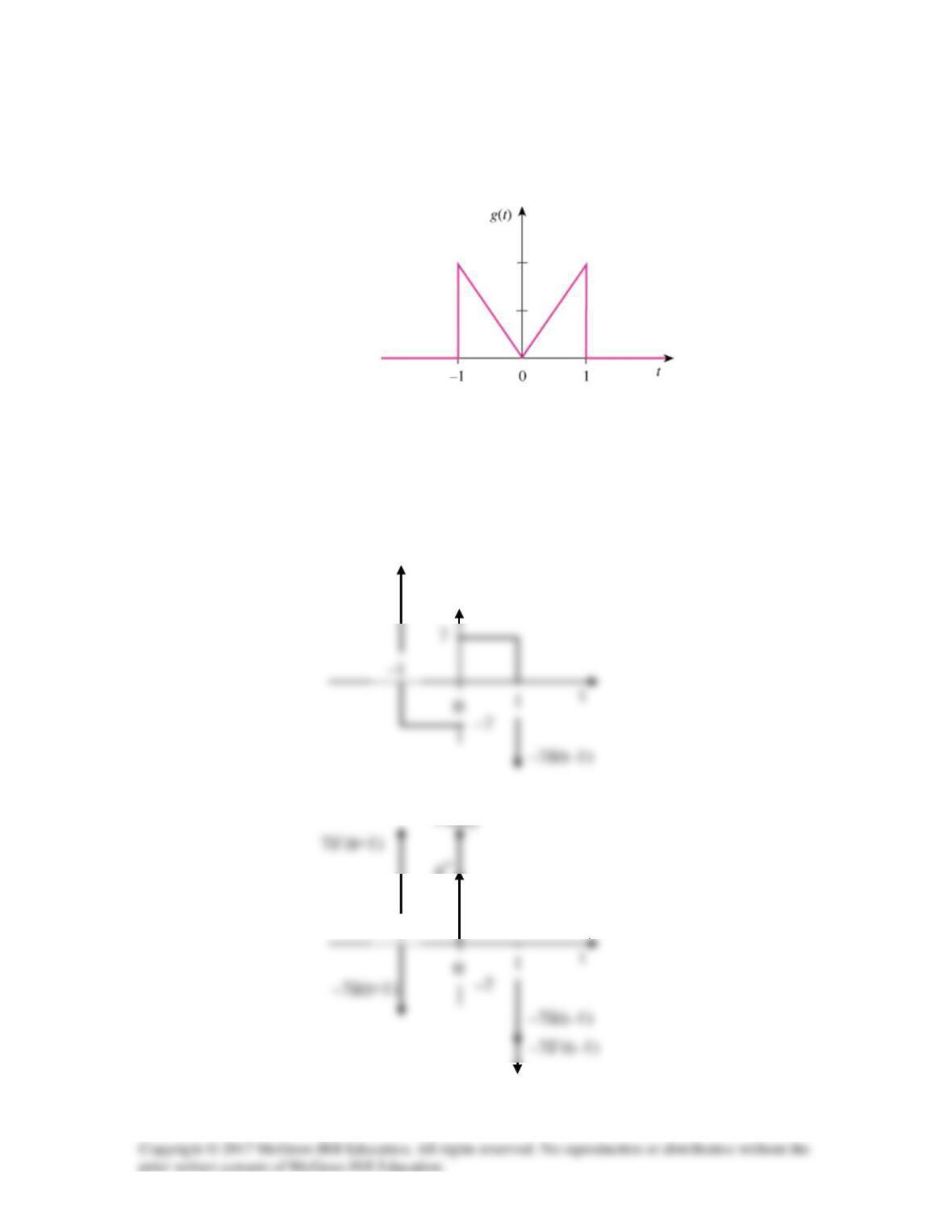
What is the Fourier transform of the triangular pulse in Fig. 18.27?
Figure 18.27
Solution
<<
1t0,t
or
∫ω−
=ω 1
0
tj dtet)(F
Solution 18.3
Calculate the Fourier transform of the signal in Fig. 18.28.
Figure 18.28
For Prob. 18.3.
Solution
22,4)(‘,22,4)( <<−=<<−= ttftttf
8
–8
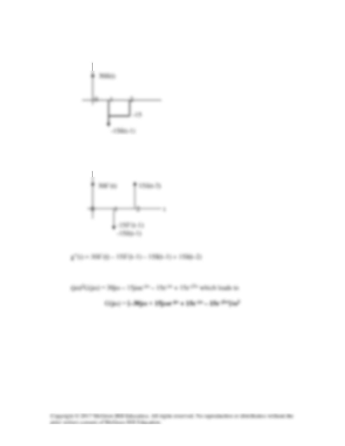
Solution 18.4
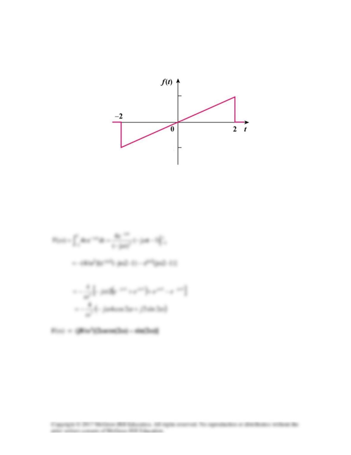
Find the Fourier transform of the waveform shown in Fig. 18.29.
Figure 18.29
For Prob. 18.4.
Solution
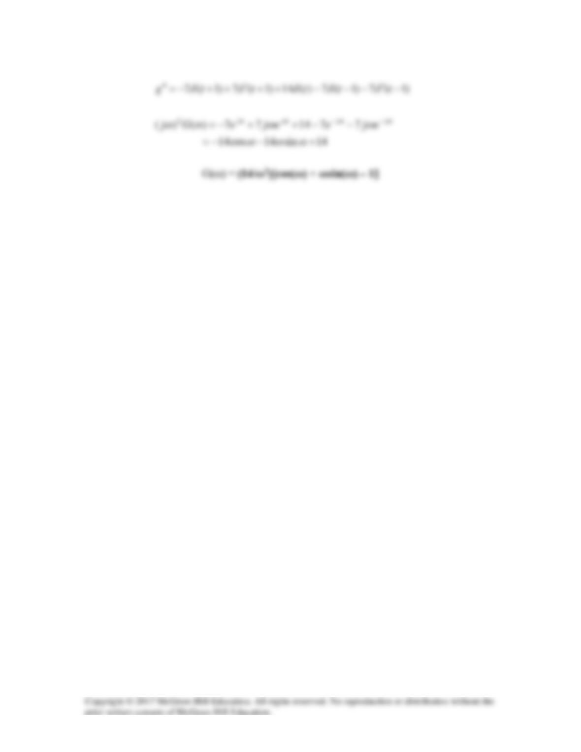
We can solve the problem by following the approach demonstrated in Example 18.5.
t
–1
t
g’
7δ(t+1)
14δ(t)
g”
–1
7
Solution 18.5
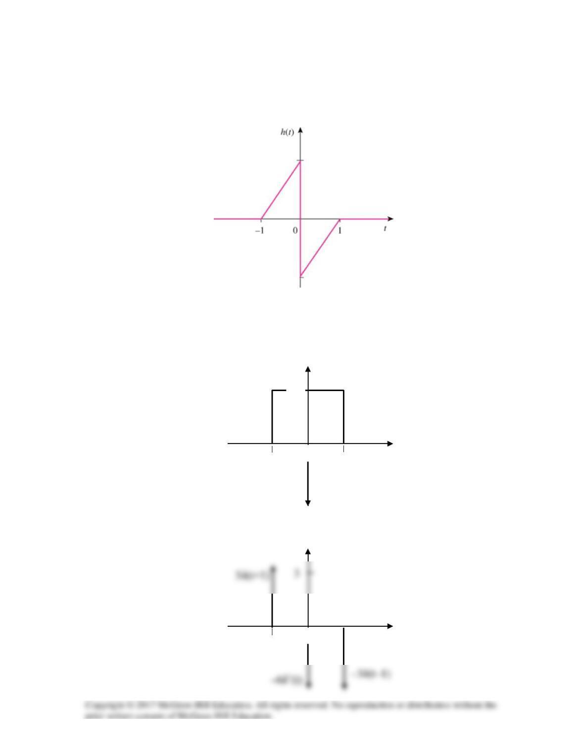
Obtain the Fourier transform of the signal shown in Fig. 18.30.
Figure 18.30
For Prob. 18.5.
Solution
3
3δ(t+1)
t
1
–1
h”(t)
0
t
1
–6δ(t)
–1
h’(t)
0
3
3
–3
δδδ
tttth
)(6)1(3)1(3)(
′
−−−+=
′′
Solution 18.6
Find the Fourier transform of each of the functions in Fig. 18.31.
f(t) g(t)
30 30
15 15
0 1 2 t 0 1 2 t
(a) (b)
Figure 18.31
For Prob. 18.6.
Solutions
(a) The derivative of f(t) is shown below.
f’(t)
15δ(t) 15δ(t-1)
0 1 2 t
(b) The derivative of g(t) is shown below.
g’(t)
The second derivative of g(t) is shown below.
g’’(t)
Take the Fourier transform of each term.
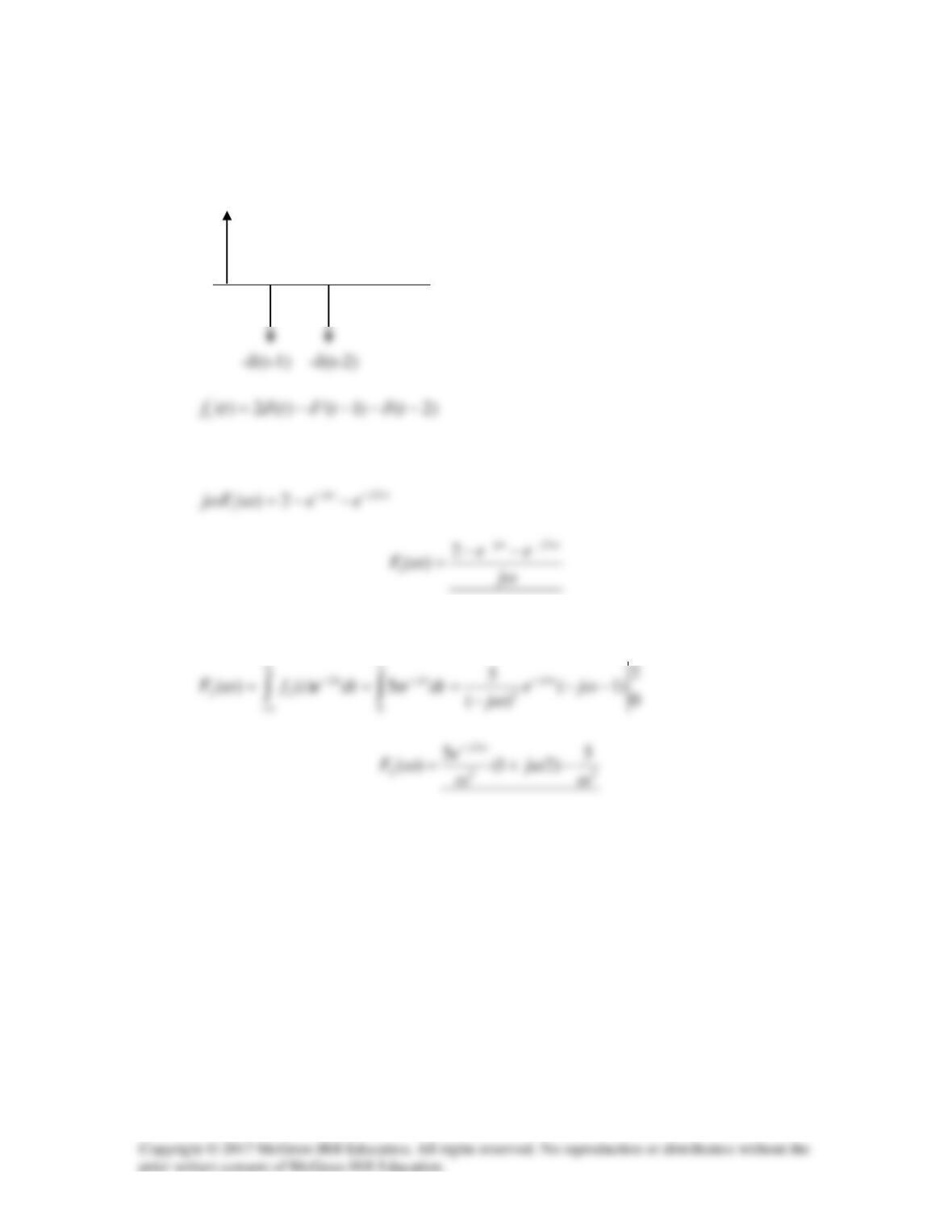
Solution 18.7
(a) Take the derivative of f1(t) and obtain f1’(t) as shown below.
2δ(t)
0 1 2 t
Take the Fourier transform of each term,
(b) f2(t) = 5t
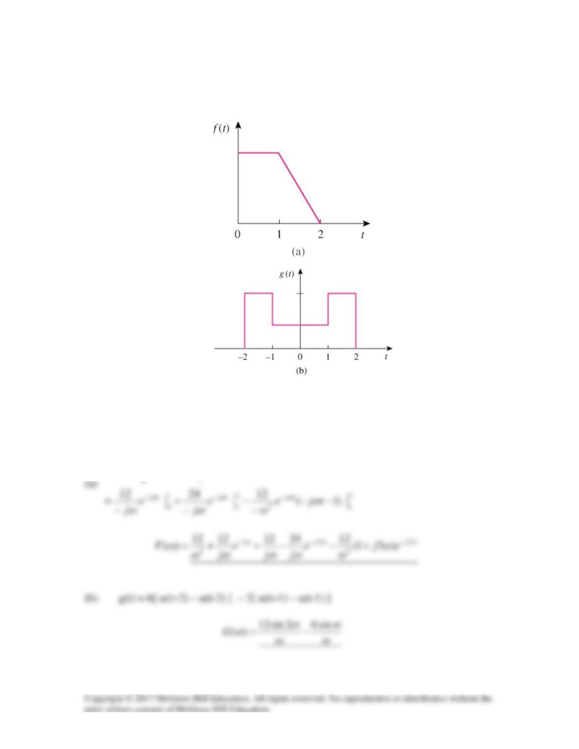
Solution 18.8
Obtain the Fourier transforms of the signals in Fig. 18.33.
Figure 18.33
For Prob. 18.8.
Solution
2
1
)1224(12)(
−+=
−−
∫∫
dtetdteF
tjtj
ω
ωω
12
6
3
Solution 18.9
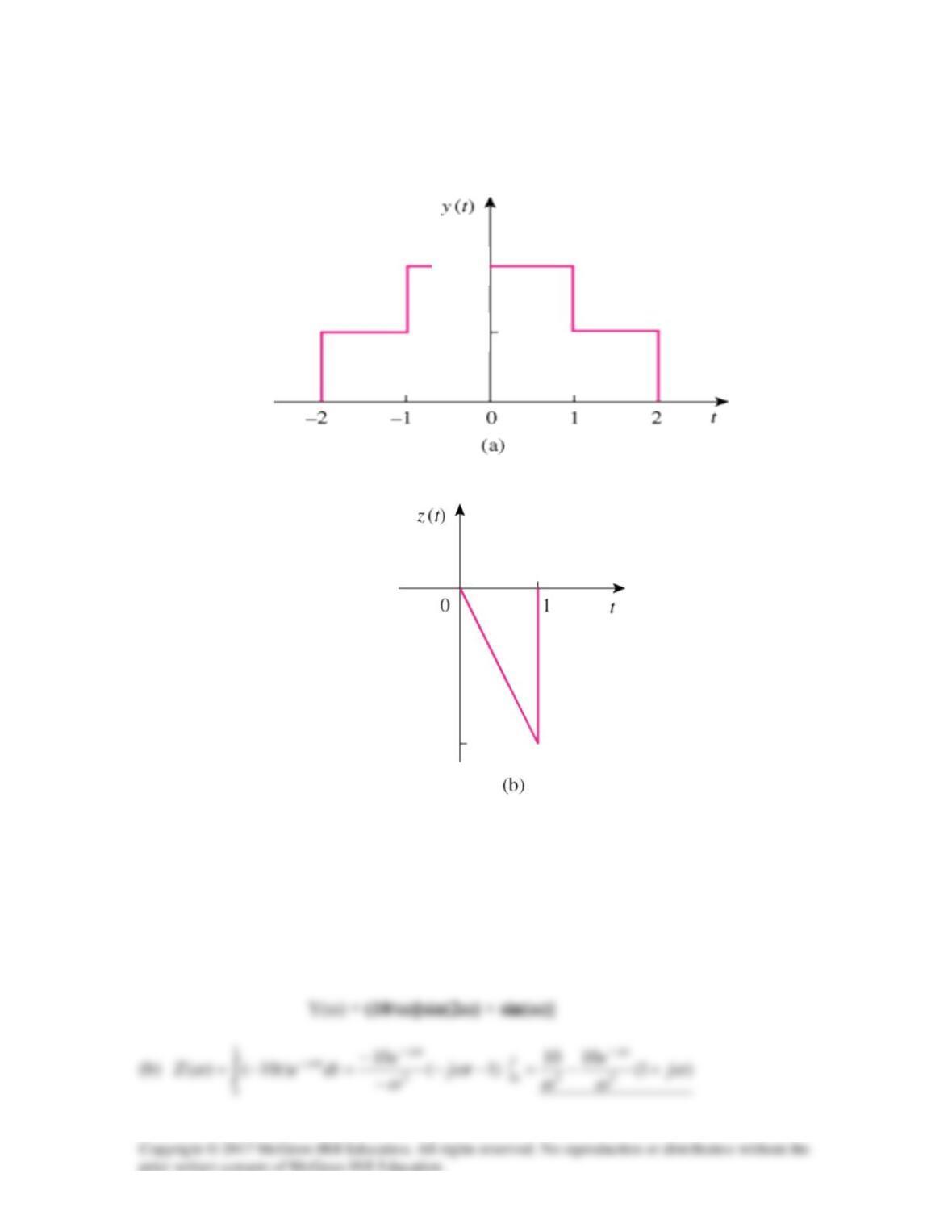
Determine the Fourier transforms of the signals in Fig. 18.34.
Figure 18.34
For Prob. 18.9.
Solution
(a) y(t) = 5u(t+2) – 5u(t–2) + 5[ u(t+1) – u(t–1) ]
10
5
–10
Solution 18.10
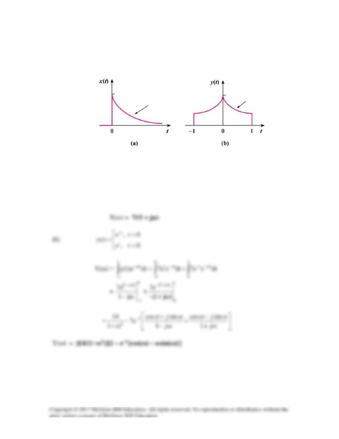
Obtain the Fourier transforms of the signals shown in Fig. 18.35.
Figure 18.35
For Prob. 18.10.
Solution
(a) x(t) = 7e–tu(t)
7
7
7e–|t|
7e–t
Solution 18.11
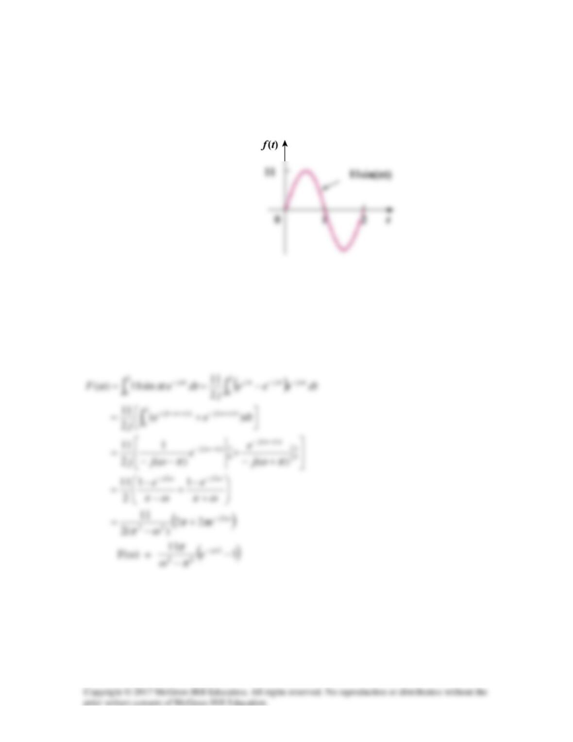
Find the Fourier transform of the “sine-wave pulse” shown in Fig. 18.36.
Figure 18.36
For Prob. 18.11.
Solution
f(t) = 11sin π t [u(t) – u(t – 2)]
Solution 18.12
Solution 18.13
(a) We know that
)]a()a([]at[cos +ωδ+−ωδπ=F
.
(b)
tsinsintcoscostsin)1t(sin π−=ππ+ππ=+π
(c ) Let y(t) = 1 + Asin at, then
)]a()a([Aj)(2)(Y −ωδ−+ωδπ+ωπδ=ω
Solution 18.14
Design a problem to help other students to better understand finding the Fourier
transform of a variety of time varying functions (do at least three).
Although there are many ways to solve this problem, this is an example based on the
same kind of problem asked in the third edition.
Problem
Find the Fourier transforms of these functions:
(a) f(t) = e-t cos (3t +
π
) u(t)
(b) g(t) = sin
π
t [ u(t + 1) – u(t–1)]
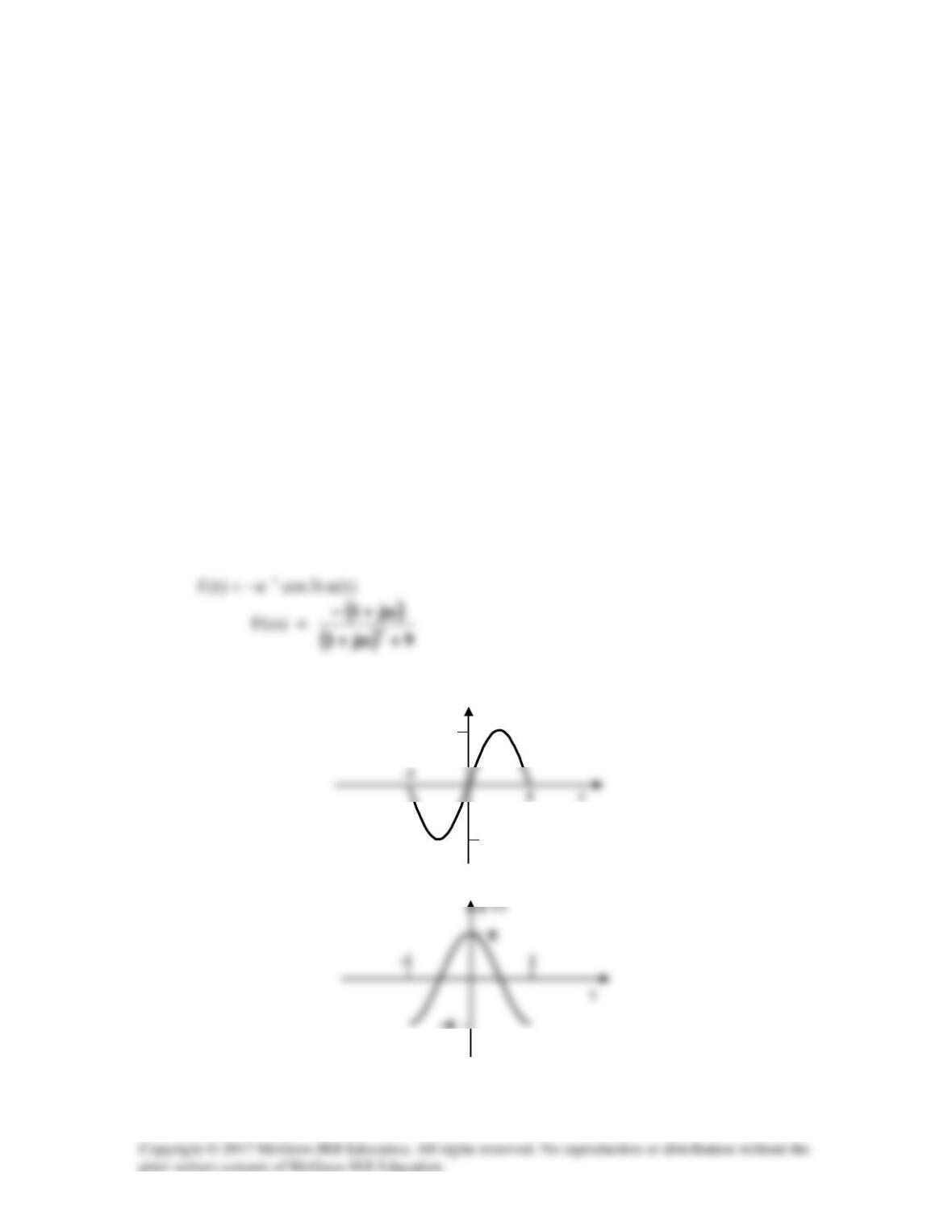
(c) h(t) = e-2t cos
π
t u(t-1)
(d) p(t) = e-2t sin 4t u(-t)
(e) q(t) = 4 sgn (t – 2) + 3
δ
(t) – 2 u(t – 2)
Solution
(a)
)t3cos()0(t3
sin)1(t3cossint3sincost3cos)t3cos( −=−−=π−π=π+
(b)
-1
-1
–π
1
-1
g(t)
[ ]
)1t(u)1t(utcos)t(‘g −−−ππ=
Alternatively, we compare this with Prob. 17.7
f(t) = g(t – 1)
(c)
tcos)0(tsin)1(tcossintsincostcos)1t(cos π−=π+−π=ππ+ππ=−π
and
)t(u)tcos(e)t(y t2 π= −
22
)j2(
j2
)(Y π+ω+
ω+
=ω
(d) Let
)t(y)t(u)t4sin(e)t(x
t2
−=−−=
−
(e)
2j2j
e
j
1
)(23e
j
8
)(Q
ω−ω−
ω
+ωπδ−+
ω
=ω