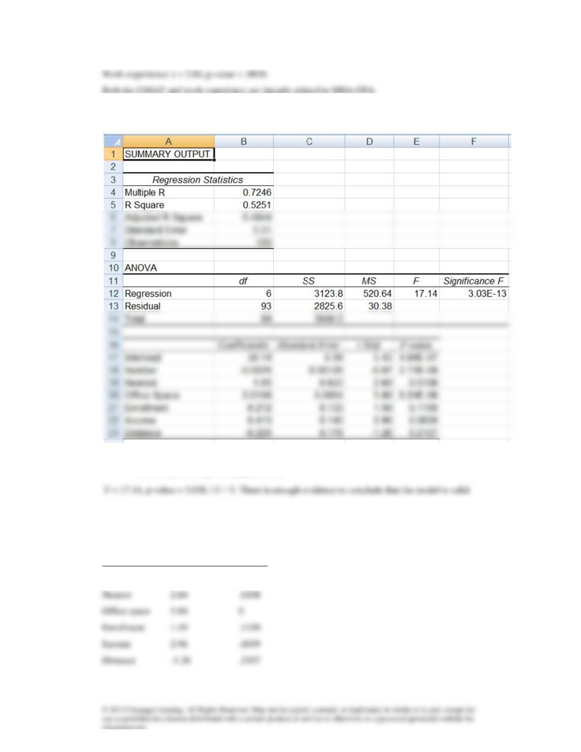
7.15
b. H0: β1 = β2 = β3 = β4 = β5 = β6 = 0
H1: At least one
is not equal to zero
c.
:H0
=i
0
:H1
i
0
Variable t-statistic p-value
Number -6.07 0
Intercept
The intercept is
0
=
b
38.14. This is the average operating margin when all the independent
Number of Motel and Hotel Rooms
The relationship between operating margin and the number of motel and hotel rooms within 3
=
b
d. Distance to Nearest Competitor
The coefficient
=
2
b
1.65 specifies that for each additional mile that the nearest competitor is to a
Office Space
The relationship between office space and operating margin is expressed by
=
3
b
.020. Because
College and University Enrollment
The relationship between operating margin and college and university enrollment is described by
=
4
b
Median Household Income
The relationship between operating margin and median household income is described by
=
5
b
Distance to Downtown Core
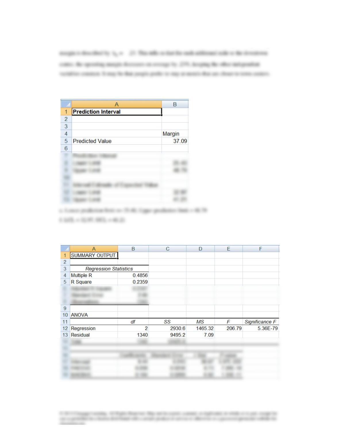
The last variable in the model is distance to the downtown core. Its relationship with operating
e. & f.
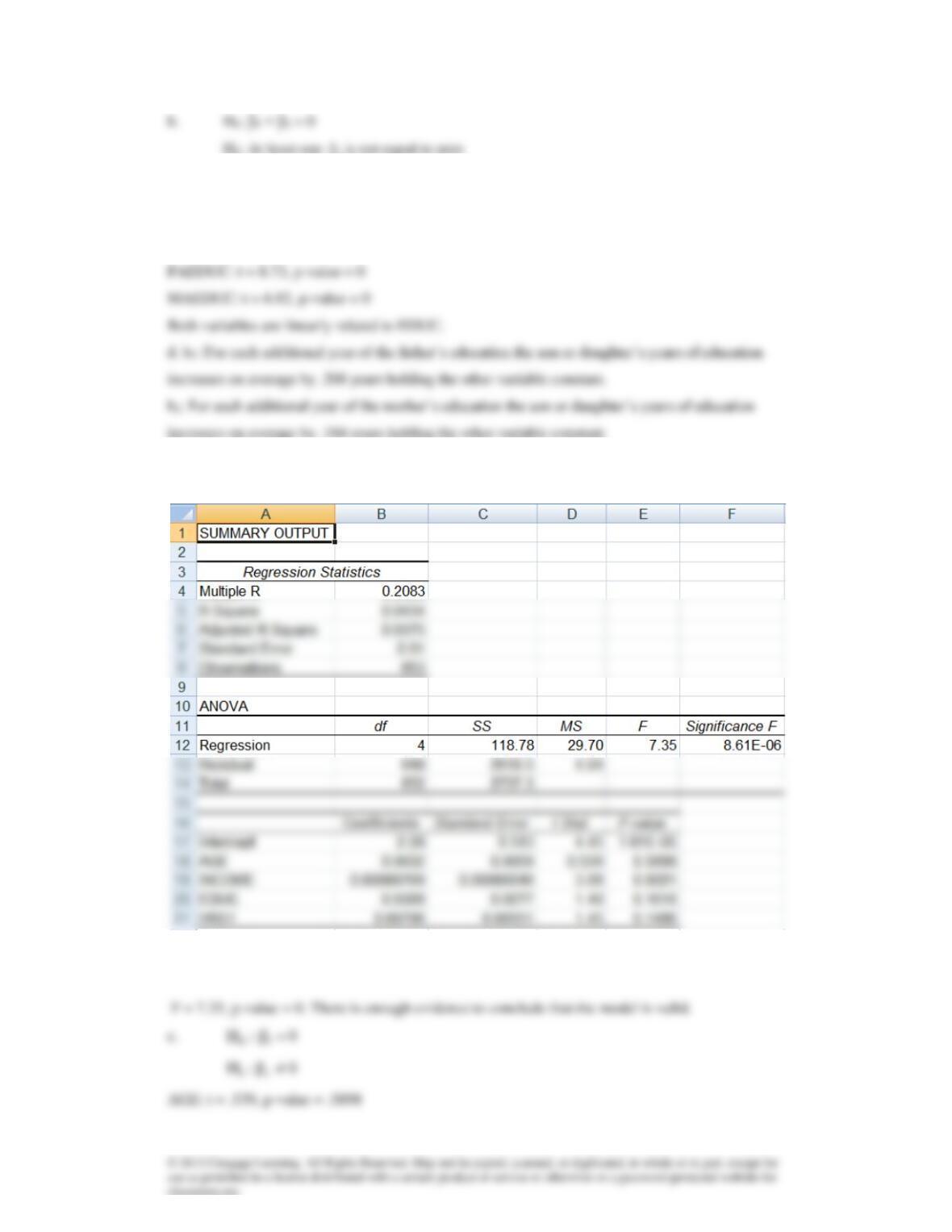
17.16
i
F = 206.79, p-value = 0. There is sufficient evidence to conclude that the model is valid.
c
:H0
=i
0
:H1
i
0
17.17
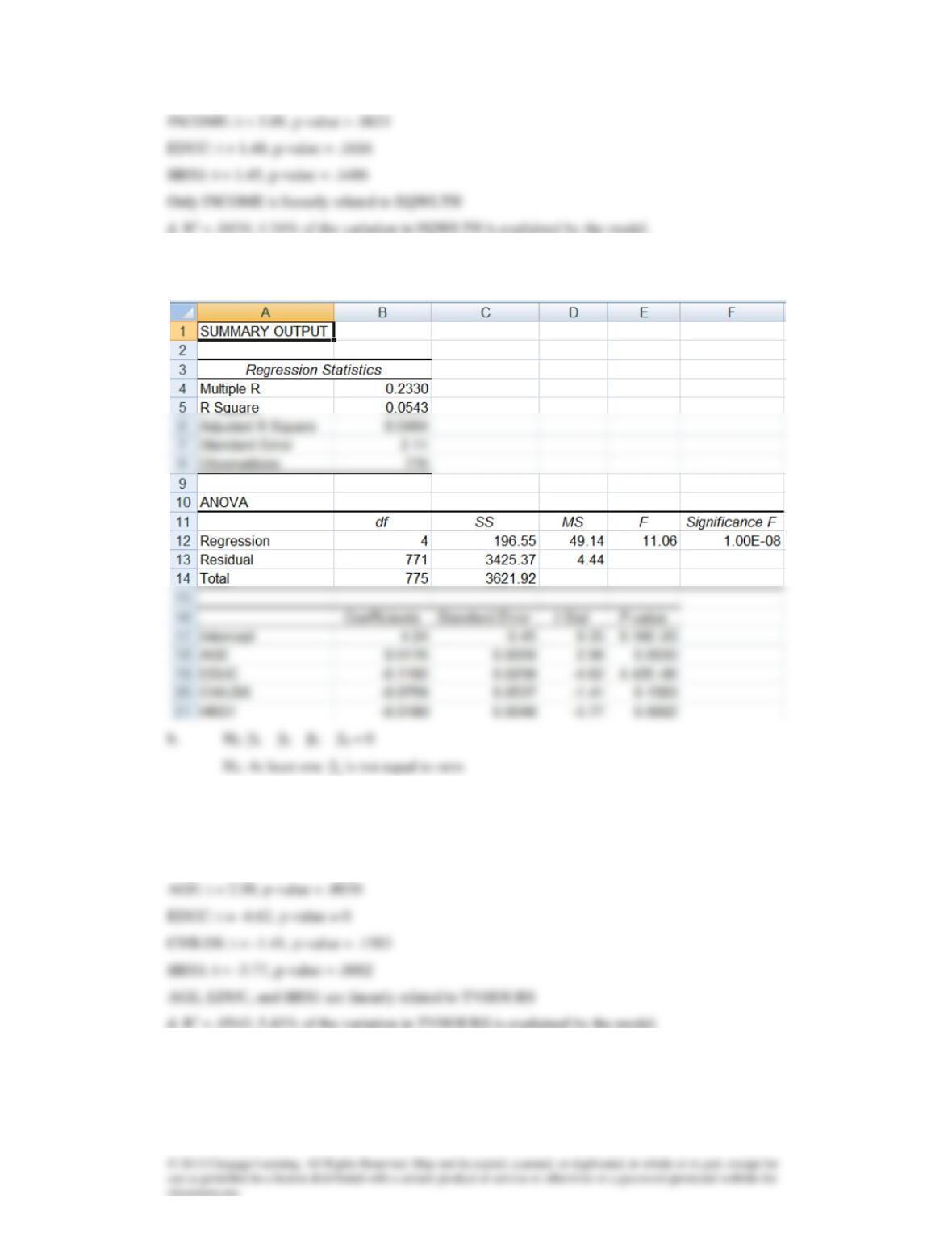
b. H0: β1 = β2 = β3 = β4 = 0
H1: At least one
i
is not equal to zero
:H0
=i
17.18
F = 11.06, p-value = 0. There is enough evidence to conclude that the model is valid.
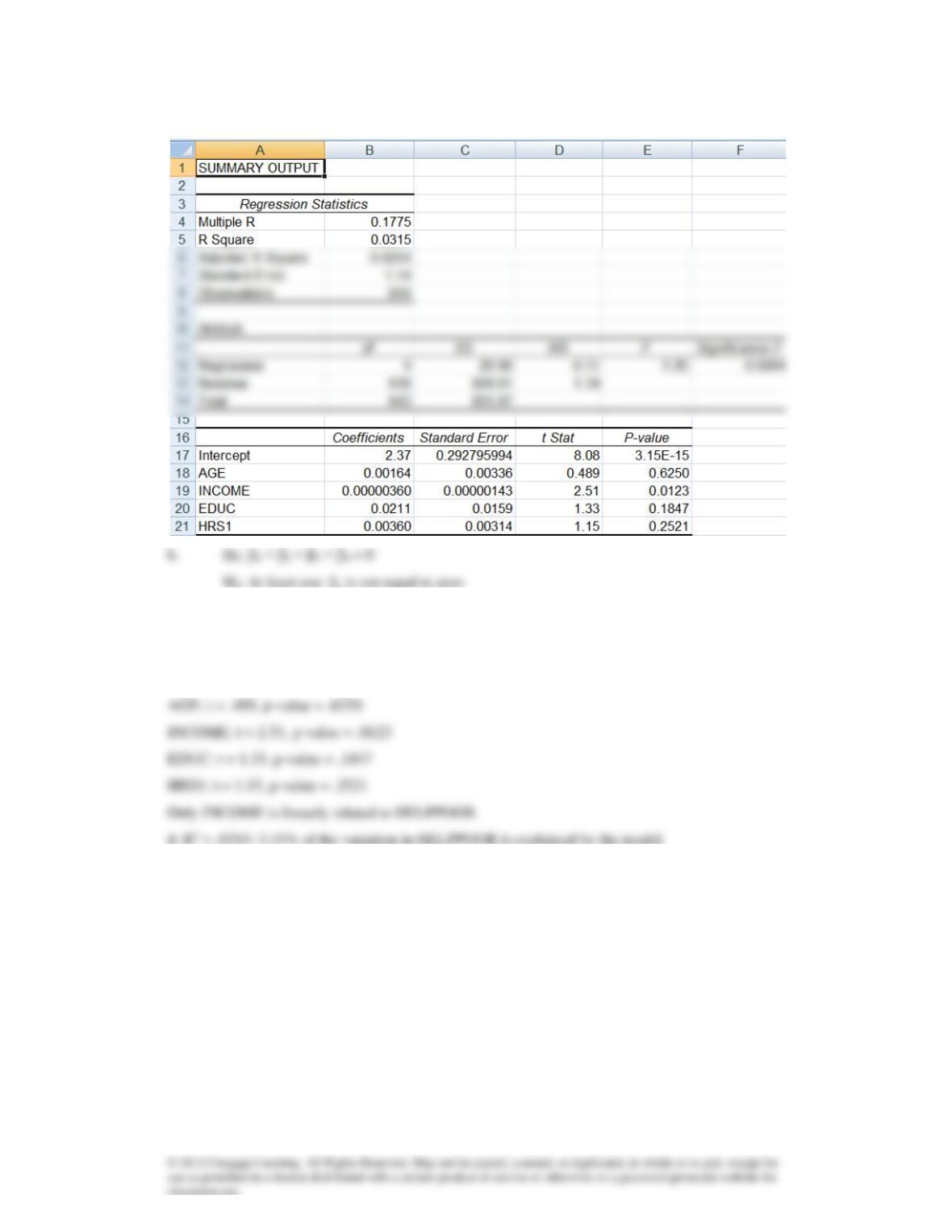
c.
:H0
=i
0
:H1
i
0
17.19
i
F = 5.20, p-value = .0004. There is enough evidence to conclude that the model is valid.
c.
:H0
=i
0
:H1
i
0
17.20
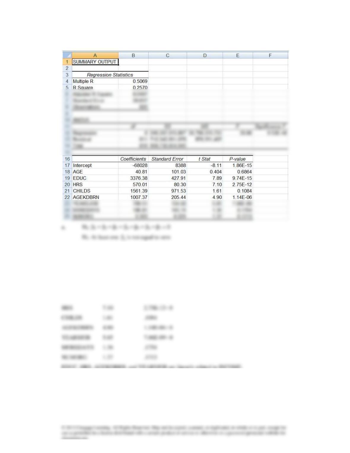
F = 35.06, p-value = 9.53E-48 ≈ 0. There is enough evidence to infer that the model is valid.
b. H0: βi = 0
H1: βi ≠ 0
Variable t-statistic p-value
AGE .40 .6864
EDUC 7.89 9.74E-15≈ 0
EDUC, HRS, AGEKDBRN, and YEARSJOB are linearly related to INCOME.
17.21
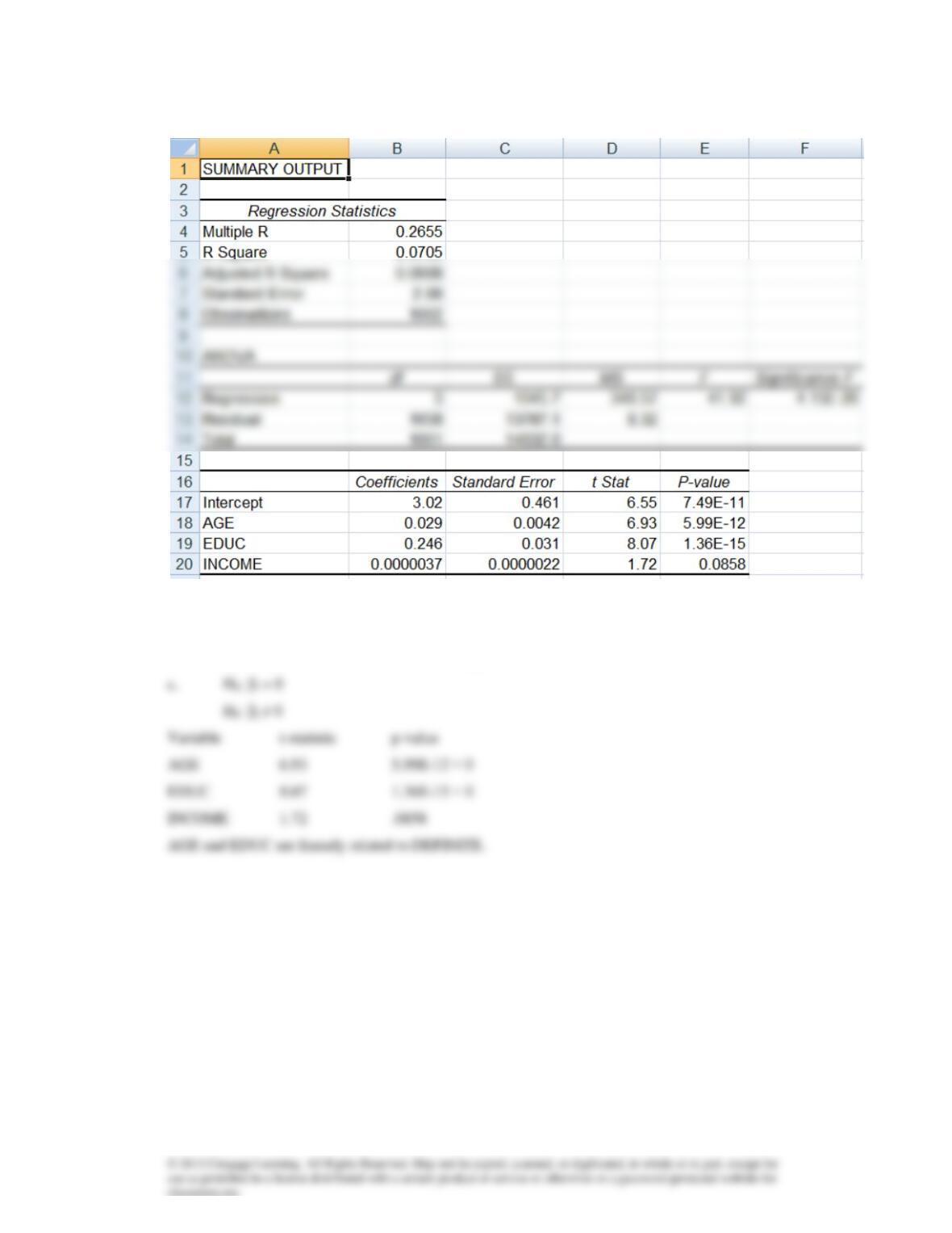
b. H0: β1 = β2 = β3 = 0
H1: At least one
i
is not equal to zero
F = 41.92, p-value = 4.15E-26 ≈ 0. There is enough evidence to infer that the model is valid.
17.22
i
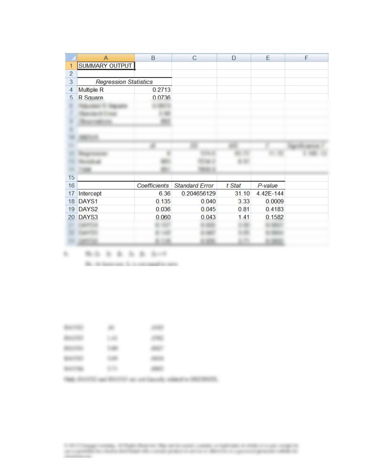
F = 11.72, p-value = 1.16E-12 ≈ 0. There is enough evidence to infer that the model is valid.
c. H0: βi = 0
H1: βi ≠ 0
Variable t-statistic p-value
DAYS1 3.33 .0009
17.23 a
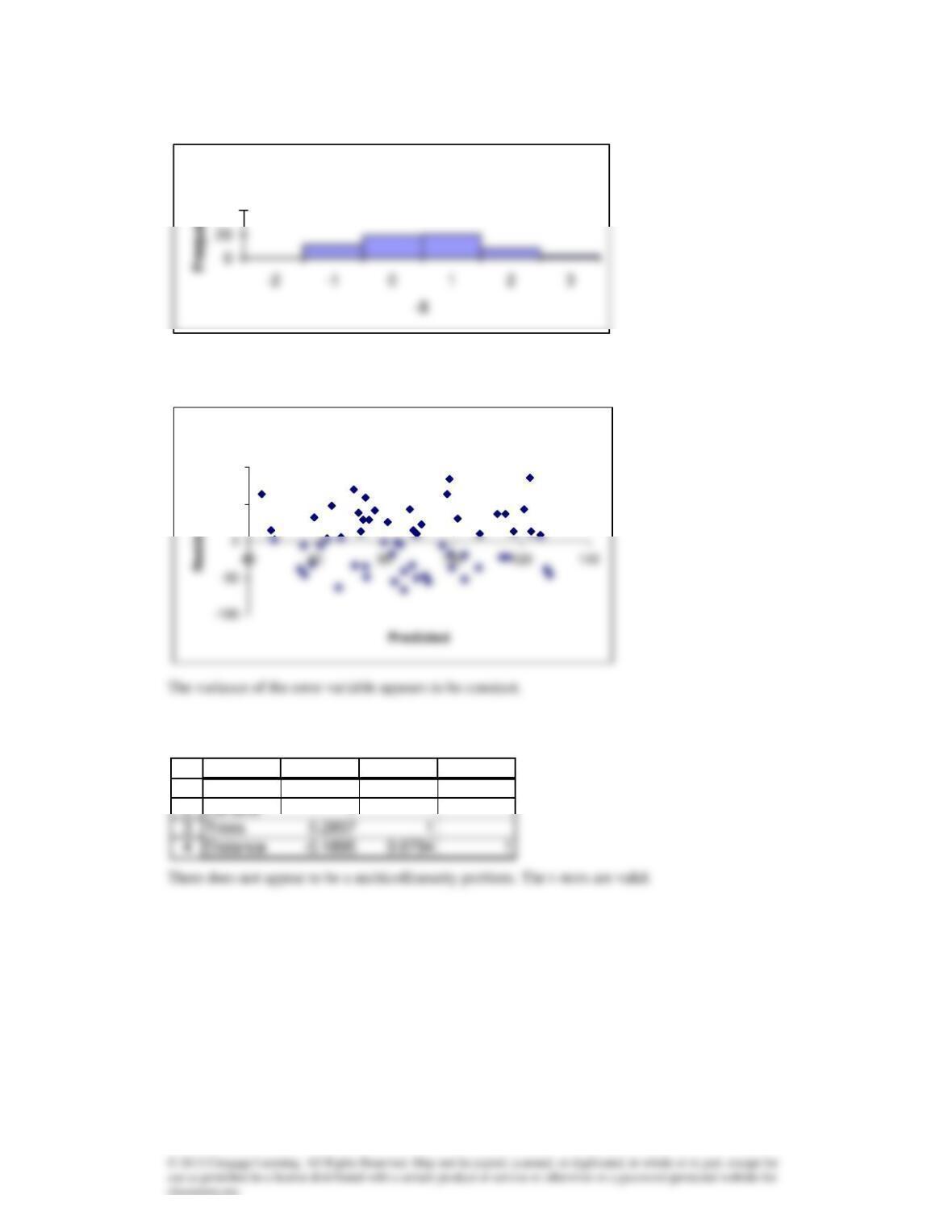
The normality requirement is satisfied.
b
17.24
Histogram
40
Plot of Residuals vs predicted
50
100
1
A B C D
Lot size Trees Distance
17.25b
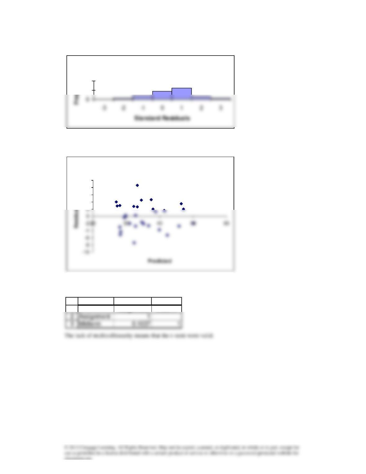
The normality requirement has not been violated.
c
The variance of the error variable appears to be constant.
d
Histogram
10
20
Plot of Residuals vs Predicted
4
6
8
10
1
A B C
Assignment Midterm
17.26a
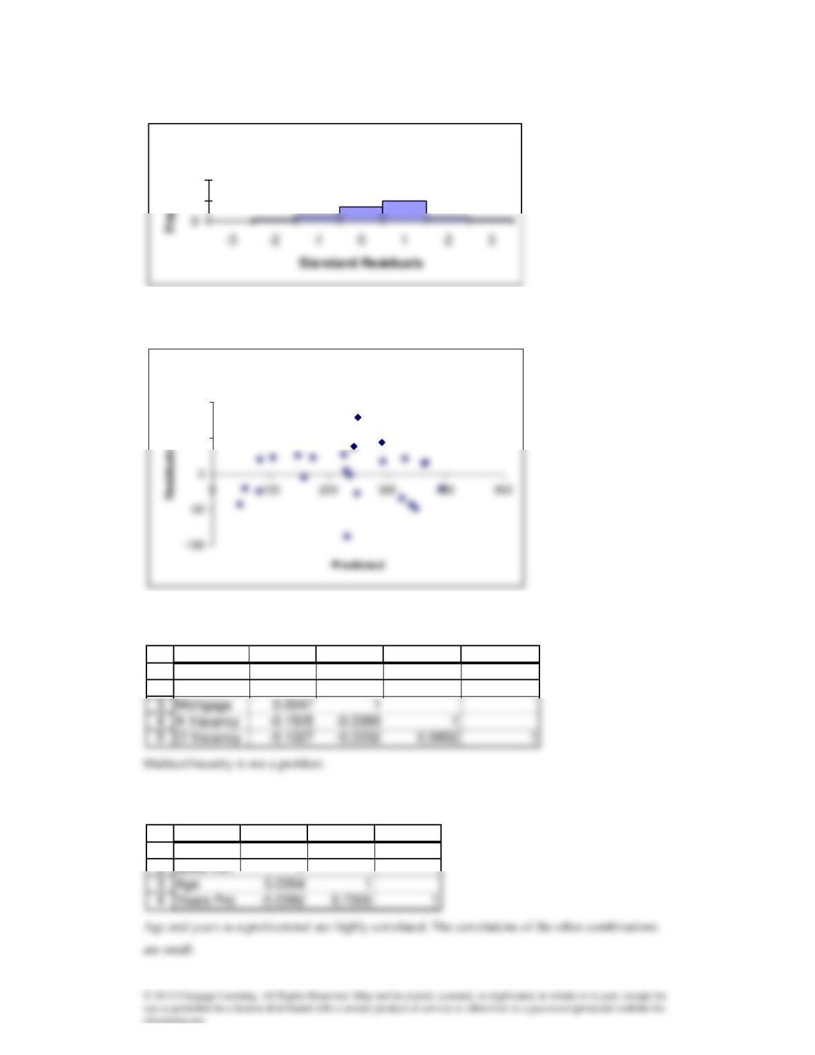
The error variable may be normally distributed.
b
The variance of the error variable is constant.
c
17.27a
Histogram
10
20
Plot of Residuals vs Predicted
50
100
1
2
A B C D E
Permits Mortgage A Vacancy O Vacancy
Permits 1
1
A B C D
Minor HR Age Years Pro
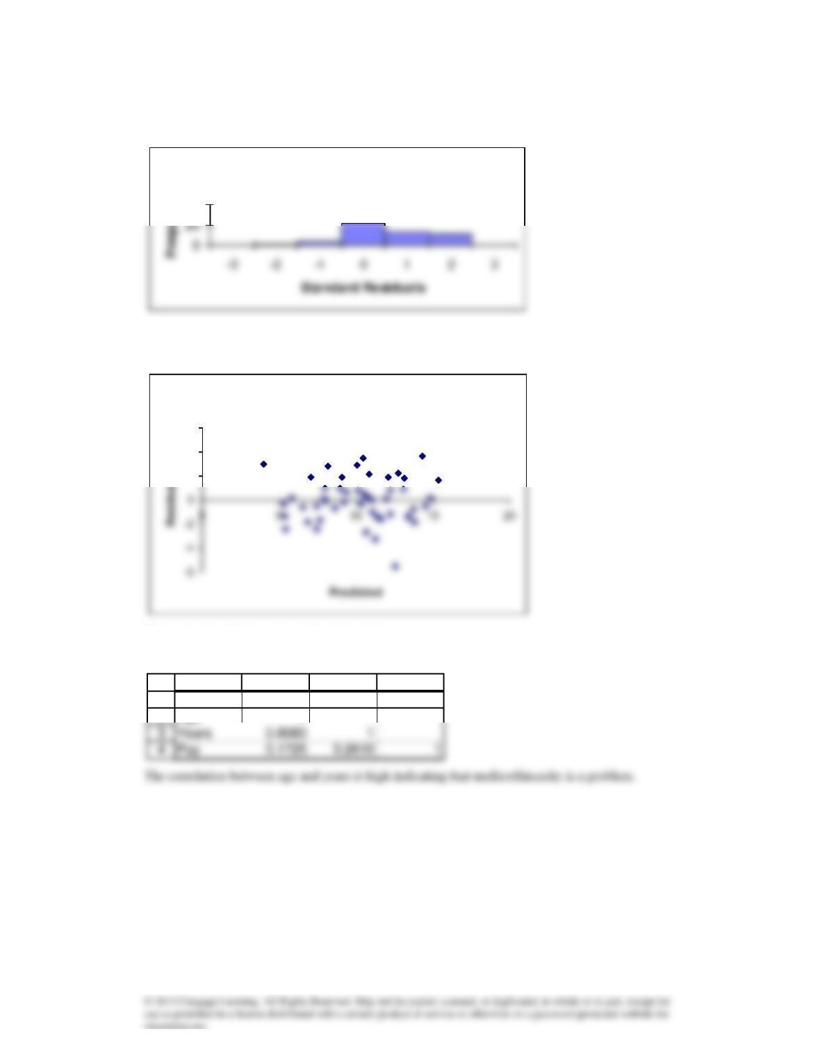
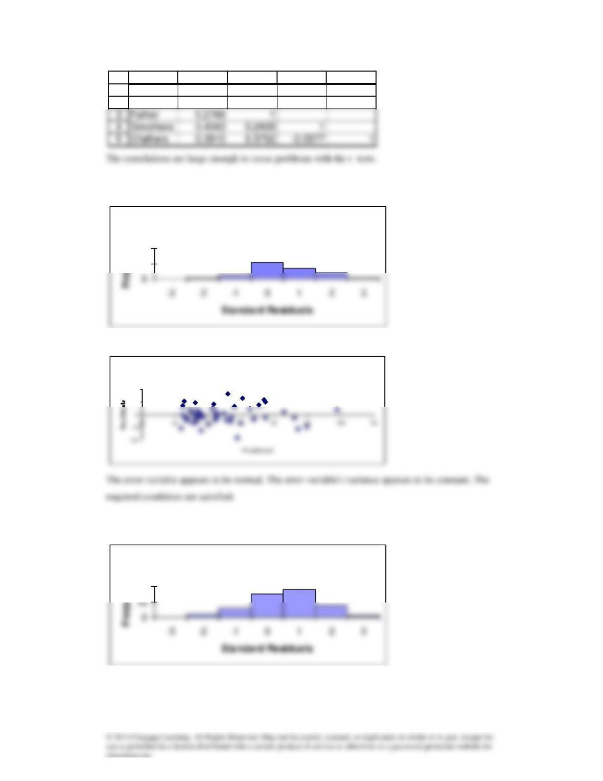
b The t–tests may not be valid.
17.28 a
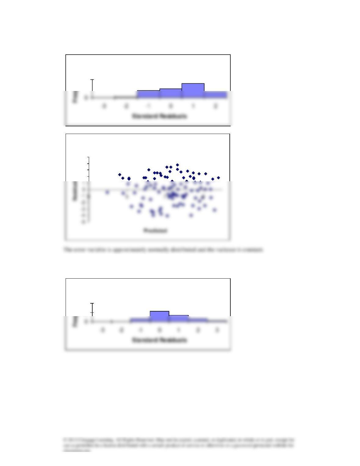
The error variable is approximately normally distributed.
b
The variance of the error variable is constant.
c
Histogram
40
Plot of Residuals vs Predicted
2
4
6
1
2
A B C D
Age Years Pay
Age 1
17.29
17.30a
Histogram
50
Plot of Residuals vs Predicted
2
3
4
5
Histogram
10
20
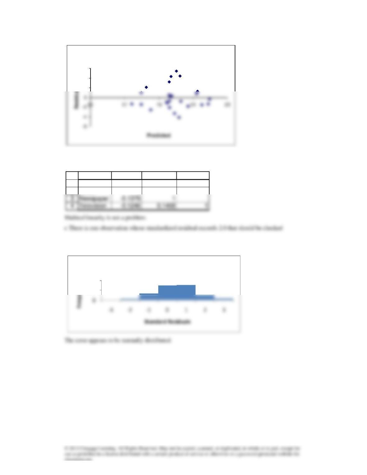
The error variable is approximately normal. However, the variance is not constant.
b
17.31
Plot of Residuals vs Predicted
2
4
6
1
2
A B C D
Direct Newspaper Television
Direct 1
100
200
Histogram
17.32 a
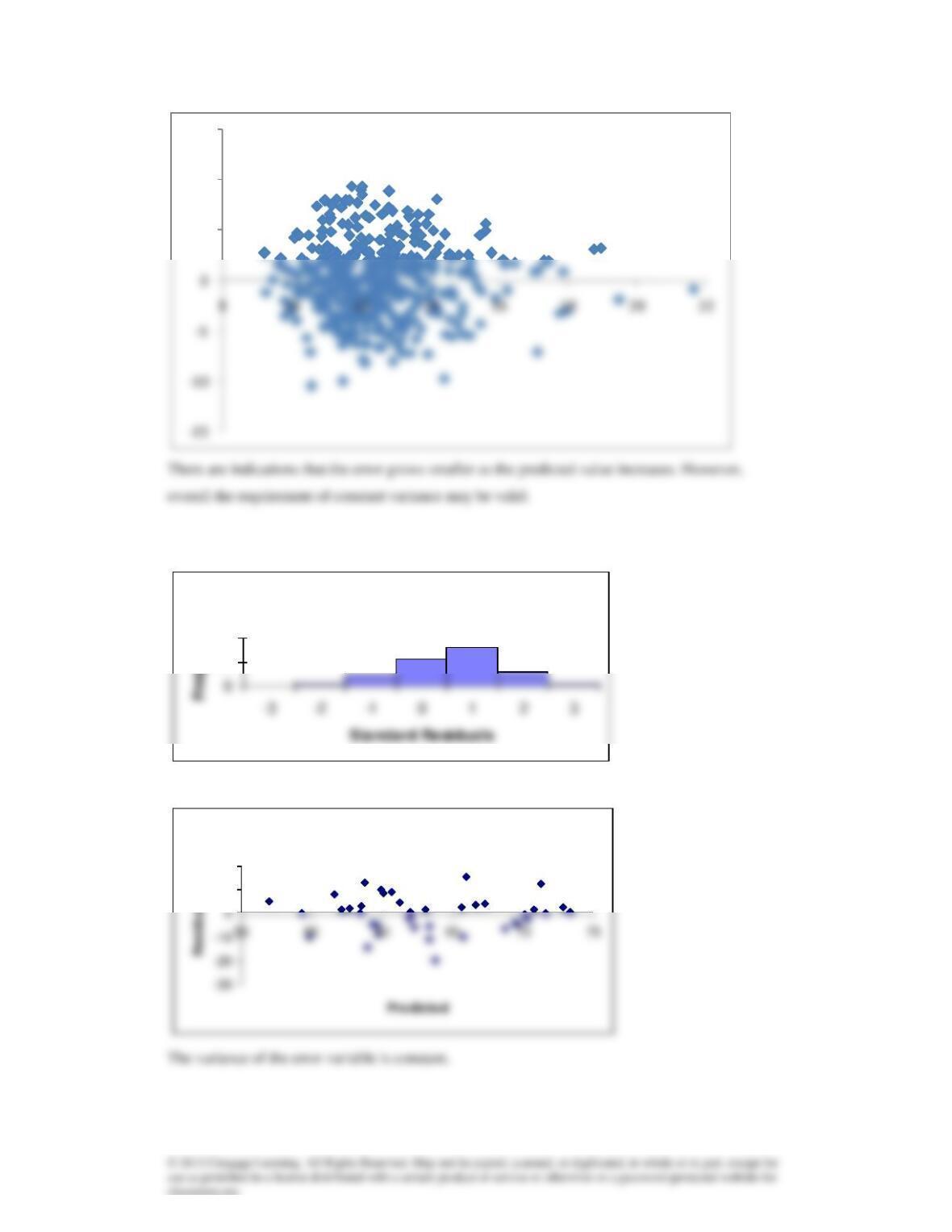
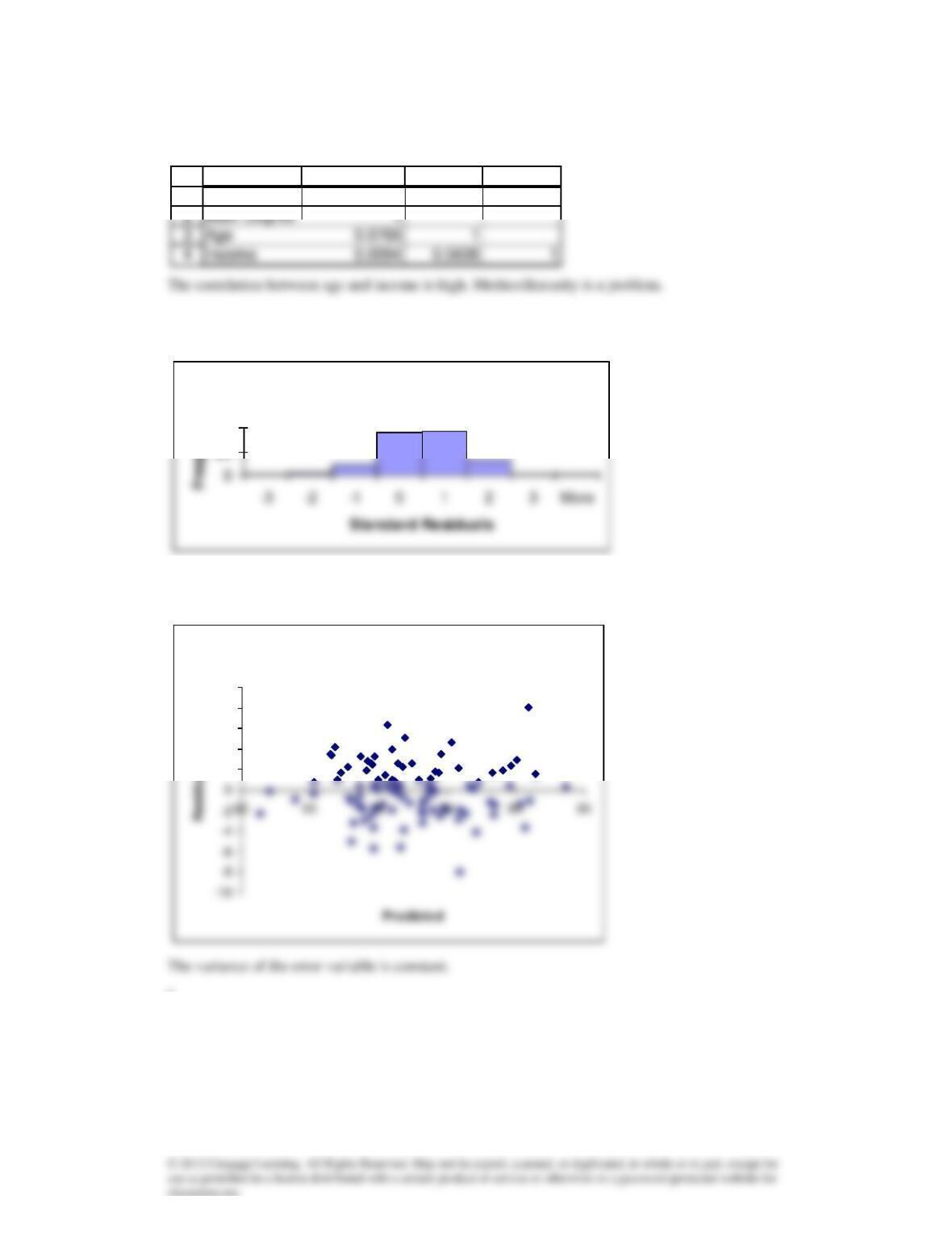
The normality requirement is satisfied.
5
10
15
Plot of Residuals vs Predicted
Histogram
10
20
Plot of Residuals vs Predicted
10
20
c
17.33a
The normality requirement is satisfied.
b
c
1
A B C D
Math Degree Age Income
Histogram
20
40
Plot of Residuals vs Predicted
2
4
6
8
10
17.34
17.35
1
2
A B C D E
Mother Father Gmothers Gfathers
Mother 1
Histogram
20
40
Plot of Residuals vs Predicted
10
20
Histogram
10
20
17.36a
Plot of Residuals vs Predicted
10
20
Histogram
40
Plot of Residuals vs Predicted
0
5
10
b
17.37
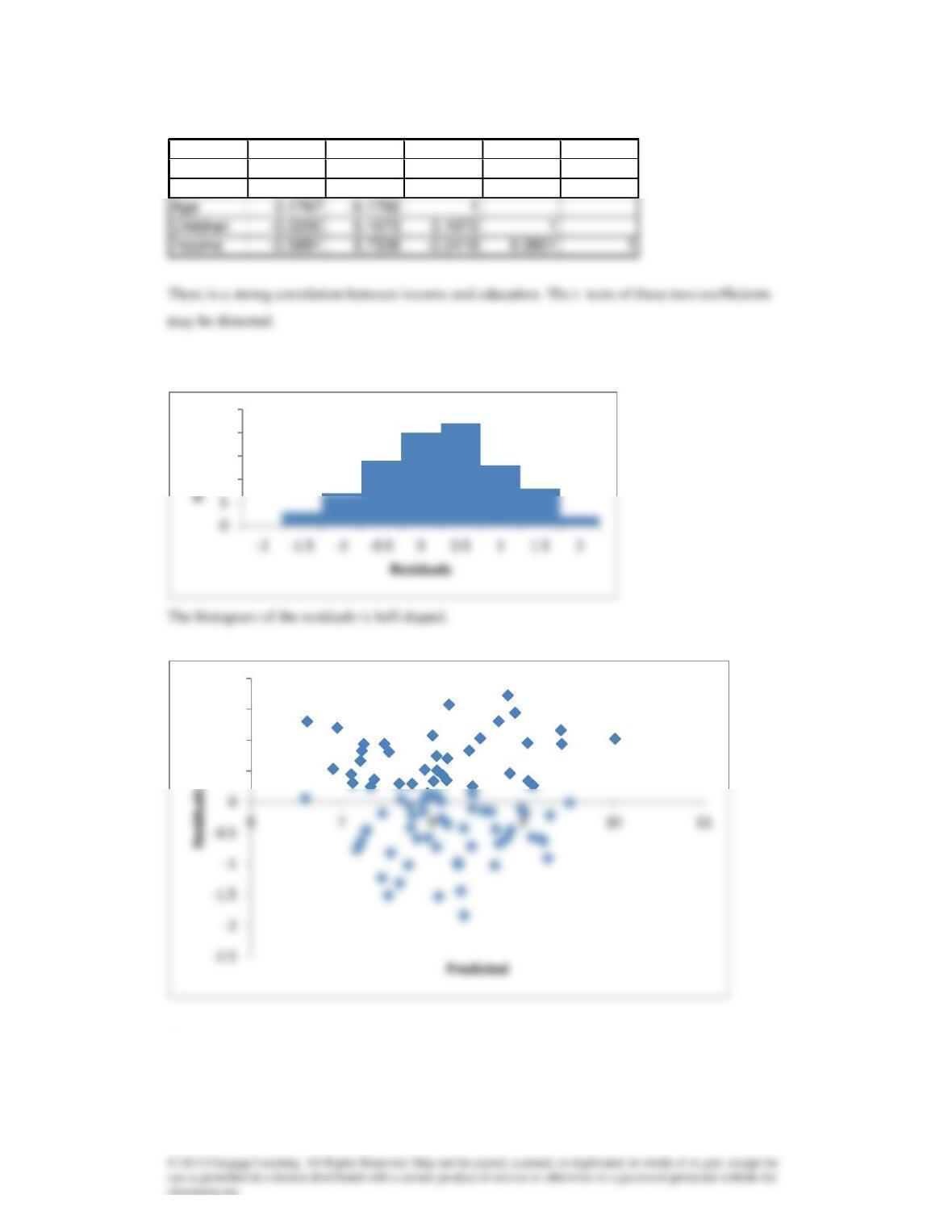
There is no evidence of heteroscedasticity.
The requirements are satisfied.
10
15
20
25
0.5
1
1.5
2
Lottery Education Age Children Income
Lottery 1
Education -0.6202 1