17.38
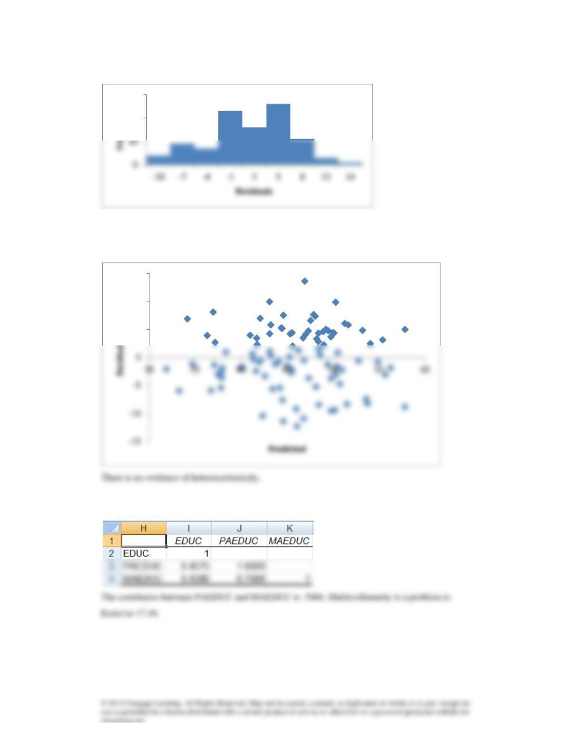
The histograms is somewhat bimodal. There residuals may not be normally distributed.
17.39
20
30
5
10
15
17.40a
b.
17.41a
17.42a
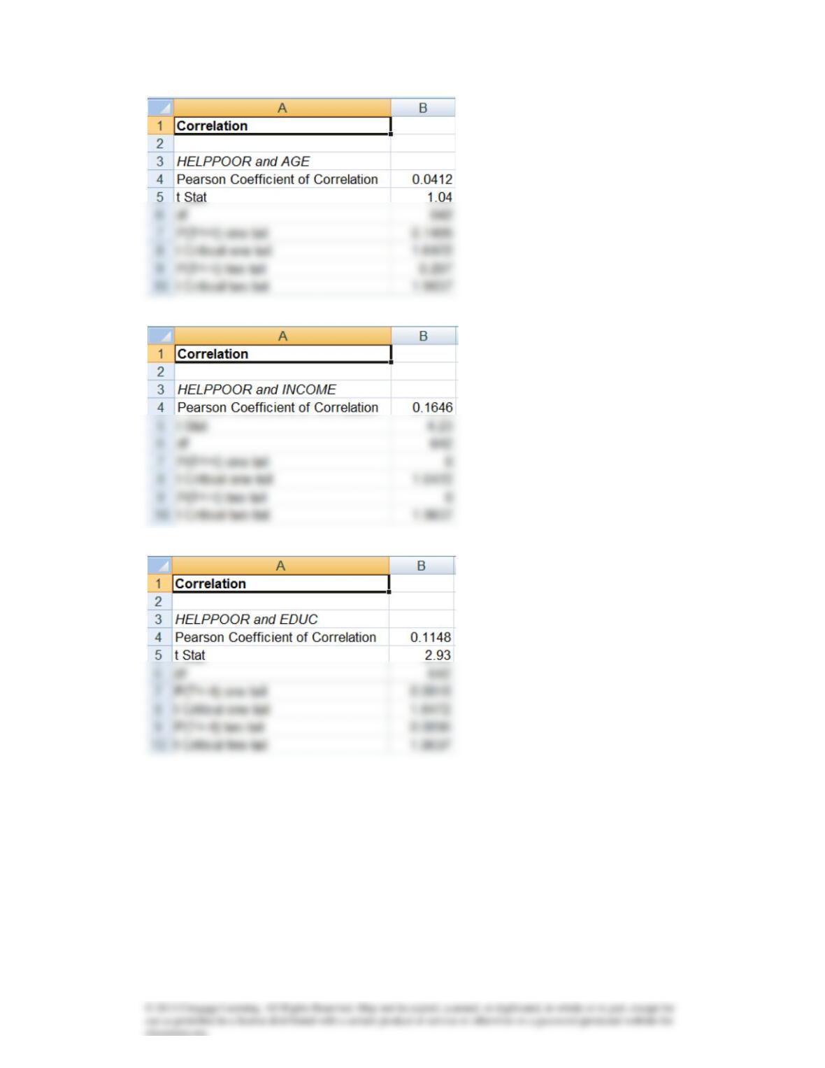
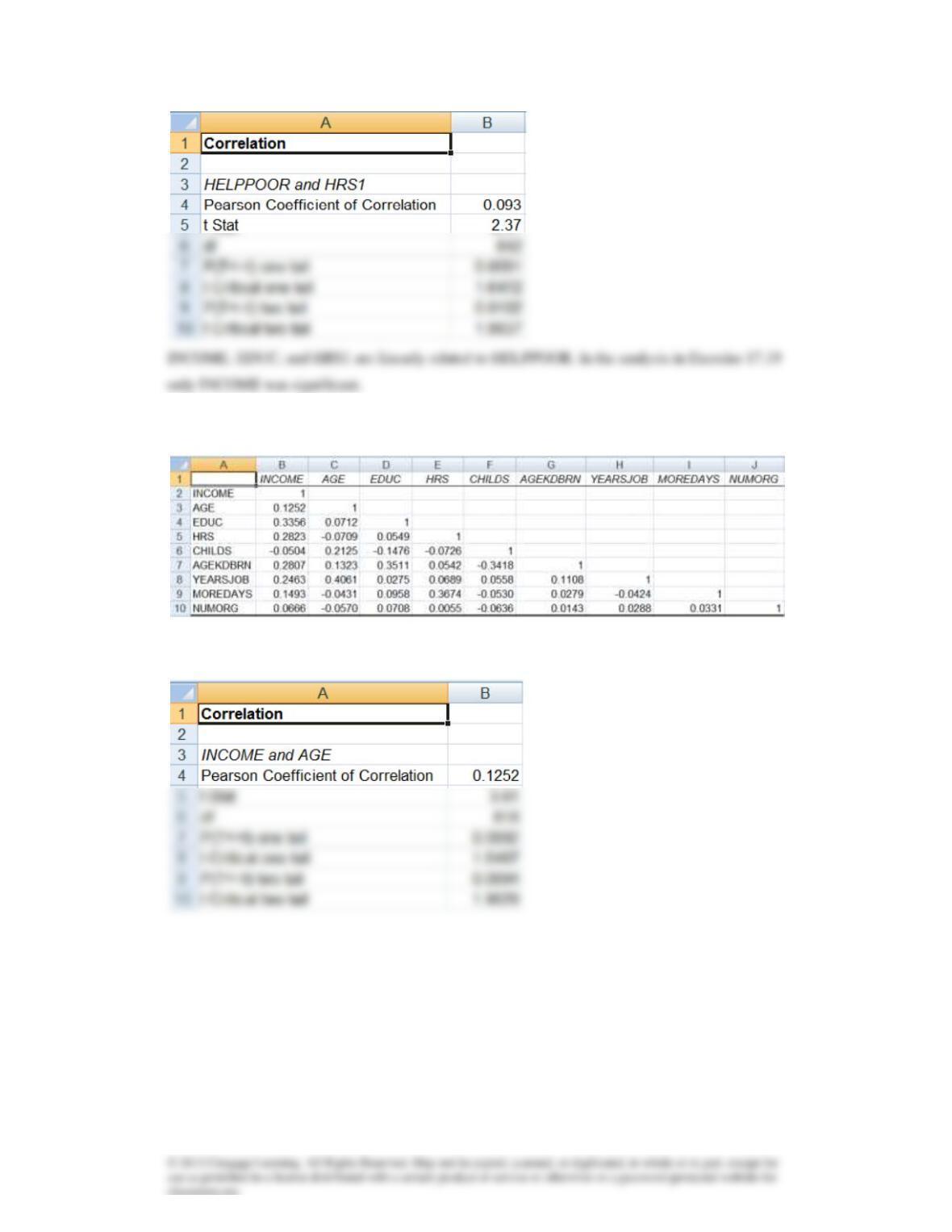
b. There are several correlations that are large enough to produce a multicollinearity effect.
c.
17.43
L
d
= 1.12,
U
d
= 1.66. There is evidence of positive first–order autocorrelation.
L
d
U
d
U
d
L
d
L
d
U
d
U
d
L
d
17.46
L
d
= 1.46,
U
d
= 1.63. There is evidence of positive first–order autocorrelation.
L
d
U
d
U
d
L
d
U
d
L
d
b
The graph indicates that autocorrelation exists.
c
e
Plot of Residuals vs Time
500
1000
1
A B C
Durbin-Watson Statistic
Plot of Residuals vs Time
200
400
600
1
A B C
Durbin-Watson Statistic
The second model fits better.
17.50 a The regression equation is
y
ˆ
= 2260 + .423x
b
There appears to be a strong autocorrelation.
c
y
ˆ
e
Plot of Residuals vs Time
500
1000
1500
1
2
A B C
Durbin-Watson Statistic
Plot of Residuals vs Time
500
1000
Tim e
17.51
17.52
order autocorrelation.
17.53 a
y
ˆ
= 898.0 + 11.33x
b
1
2
A B C
Durbin-Watson Statistic
1
2
A B C
Durbin-Watson Statistic
1
2
A B C
Durbin-Watson Statistic
Histogram
10