Appendix 17
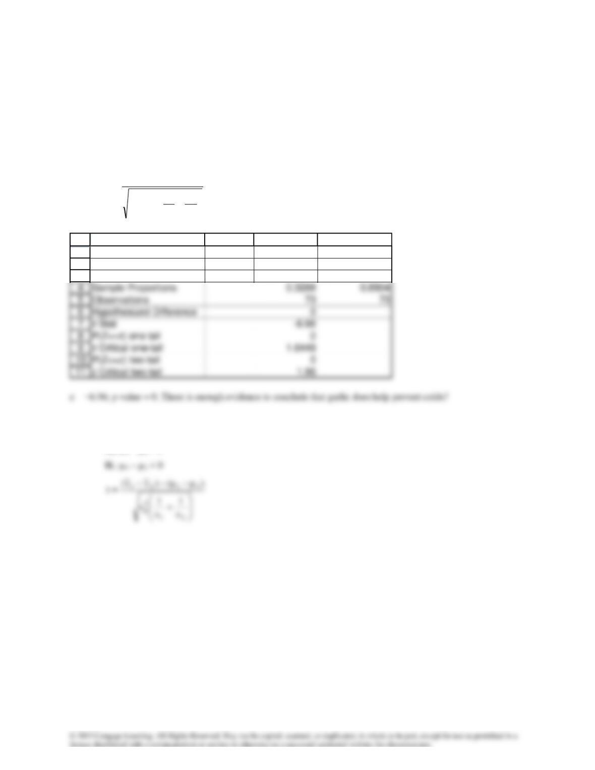
A17.1a z-test of p1 – p2 (case 1)
H0: p1 – p2 = 0
H1: p1 – p2 < 0
+−
−
=
21
21
n
1
n
1
)p
ˆ
1(p
ˆ
)p
ˆ
p
ˆ
(
z
1
2
3
A B C D
z-Test: Two Proportions
Allicin Cold? Placebo Cold?
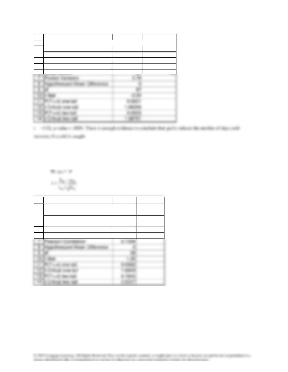
b. Equal-variances t-test of µ1 − µ2
H0: µ1 – µ2 = 0
1
2
3
4
5
6
A B C
t-Test: Two-Sample Assuming Equal Variances
Allicin Days Placebo Days
Mean 6.29 8.11
Variance 2.39 4.25
Observations 24 65
A17.2 t-test of µD
H0: µD = 0
1
2
3
4
5
6
A B C
t-Test: Paired Two Sample for Means
Eye-level Lower shelf
Mean 302.4 290.8
Variance 2482.2 6262.7
Observations 40 40
t = 1.35; p-value = .0922. There is not enough evidence to conclude that placement of the product at eye level
significantly increases sales?
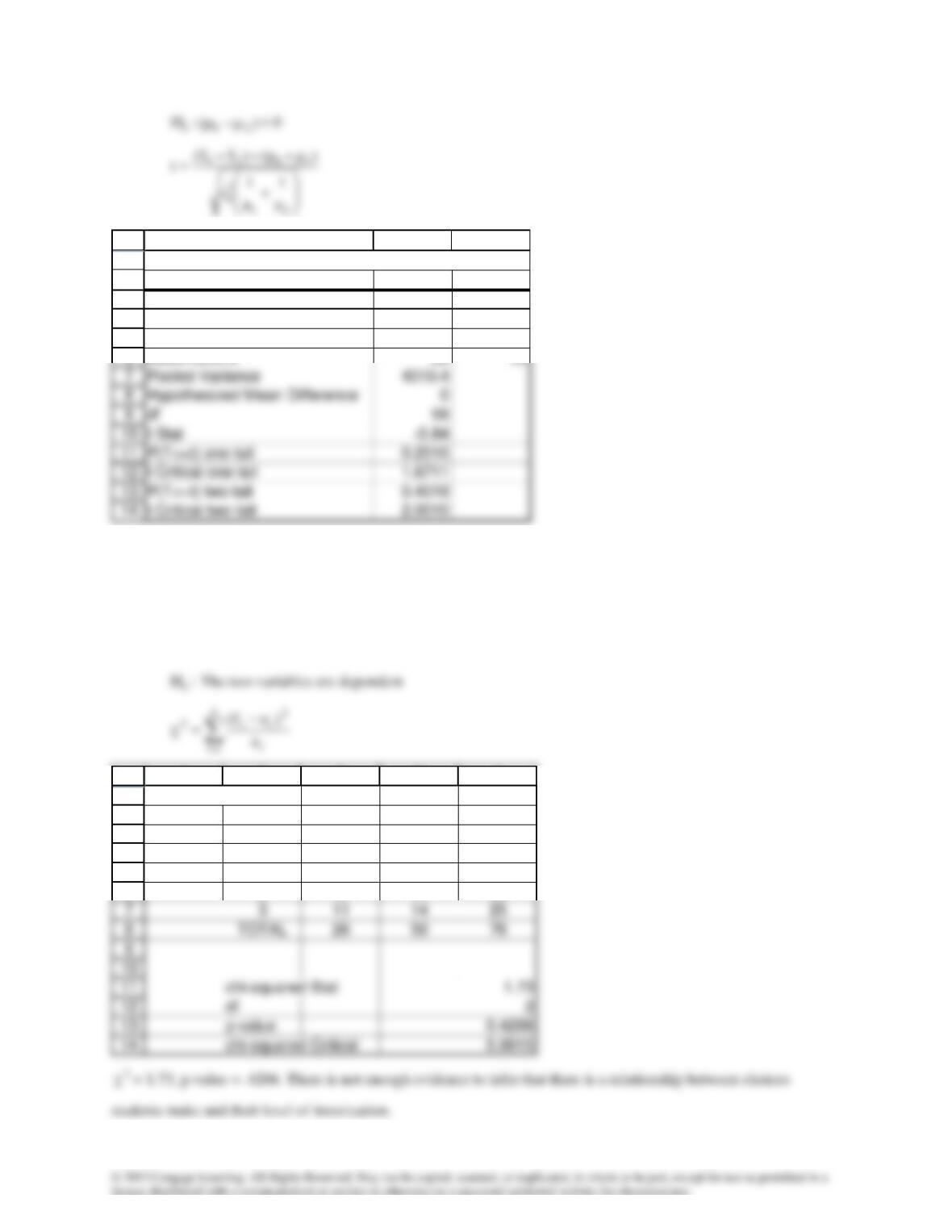
A17.3 Equal-variances t-test of
21 −
)(:H 210 −
= 0
1
2
3
4
5
6
A B C
t-Test: Two-Sample Assuming Equal Variances
British American
Mean 6344.5 6358.3
Variance 5084.0 3104.6
Observations 28 33
t = –.84, p-value = .2010. There is not enough evidence to conclude that British courses are shorter than American
courses.
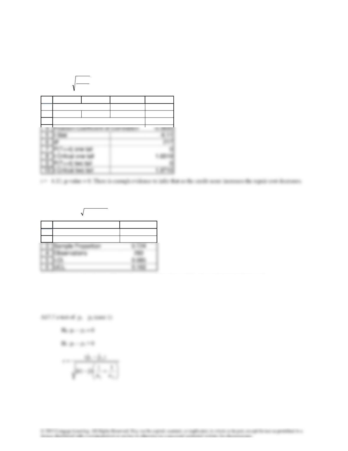
A17.4 Chi-squared test of a contingency table
:H0
The two variables are independent
1
2
3
4
5
6
A B C D E
Contingency Table
Group
Choice 1 2 TOTAL
1 7 19 26
2 8 17 25
A17.5 t-test of ρ or β1
:H
0
= 0
0:H1
2
r1
2n
rt −
−
=
1
2
3
A B C D
Correlation
Repair cost and Credit score
A17.6 z-estimator of p
n/)p
ˆ
1(p
ˆ
zp
ˆ2/ −
1
2
A B
z-Estimate: Proportion
Photography
Confidence interval estimate of the total number of American adults who participate in photography
LCL = 205.8 million (.085) = 17.493 million
UCL = 205.8 million (.162) = 33.396 million
1
2
3
4
5
A B C D
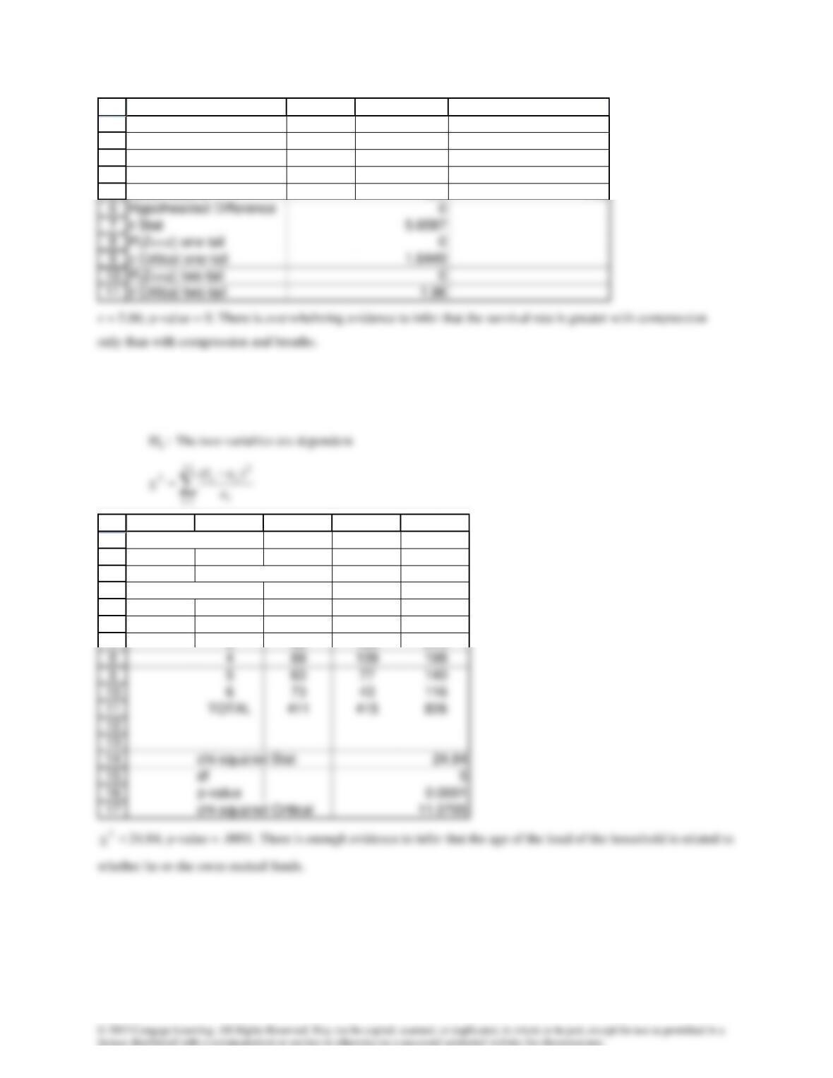
z-Test: Two Proportions
Compression Compression & breaths
Sample Proportions 0.221 0.0997
Observations 439 712
A17.8 Ch-squared test of a contingency table
:H0
The two variables are independent
1
2
3
4
5
6
7
A B C D E
Contingency Table
Age category
Mutual fund 1 2 TOTAL
119 625
275 57 132
392 123 215
A17.9 Equal-variances t-test of
21 −
)(:H 210 −
= 0
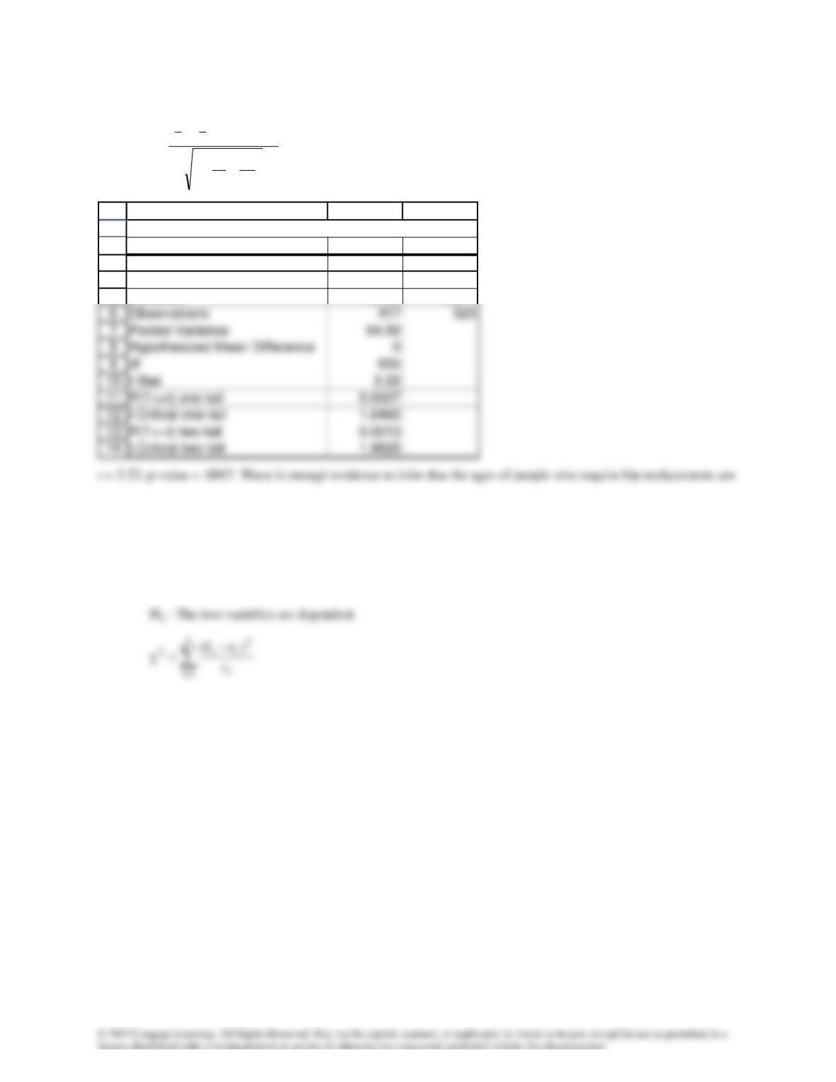
)(:H 211 −
> 0
+
−−−
=
21
2
p
2121
n
1
n
1
s
)()xx(
t
1
2
3
4
5
A B C
t-Test: Two-Sample Assuming Equal Variances
Year 1995 Year 2005
Mean 66.37 64.67
Variance 64.24 64.71
getting smaller?
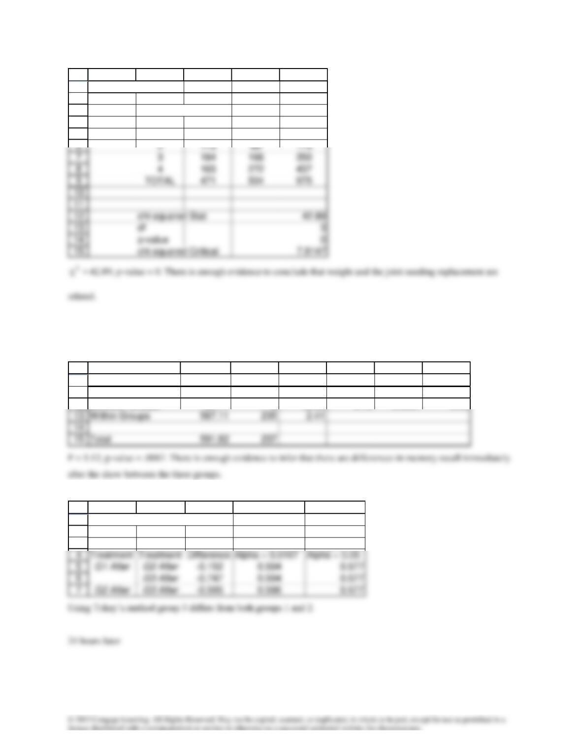
A17.10 Chi-squared test of a contingency table
:H0
The two variables are independent
1
2
3
4
5
A B C D E
Contingency Table
Weight category
Hip/Knee 1 2 TOTAL
1 9 6 15
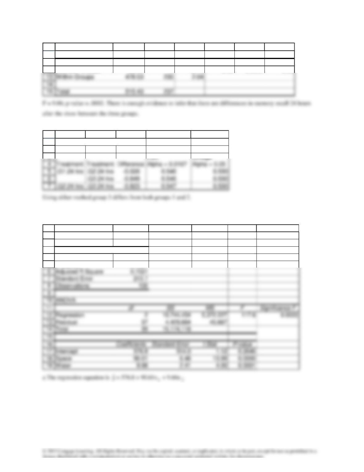
A17.11 One-way analysis of variance and multiple comparisons
After the show
10
15
11
12
A B C D E F G
ANOVA
Source of Variation SS df MS F P-value F crit
Between Groups 24.71 2 12.35 5.12 0.0067 3.03
1
2
3
A B C D E
Multiple Comparisons
LSD Omega
10
15
11
12
A B C D E F G
ANOVA
Source of Variation SS df MS F P-value F crit
Between Groups 36.90 2 18.45 9.06 0.0002 3.03
1
2
A B C D E
Multiple Comparisons
A17.12
1
2
8
3
4
5
A B C D E F
SUMMARY OUTPUT
Regression Statistics
Multiple R 0.8415
R Square 0.7081
b The coefficient of determination is
2
R
= .7081; 70.81% of the variation in electricity consumption is explained by
the model. The model fits reasonably well.
c
:H0
=1
=2
0
i
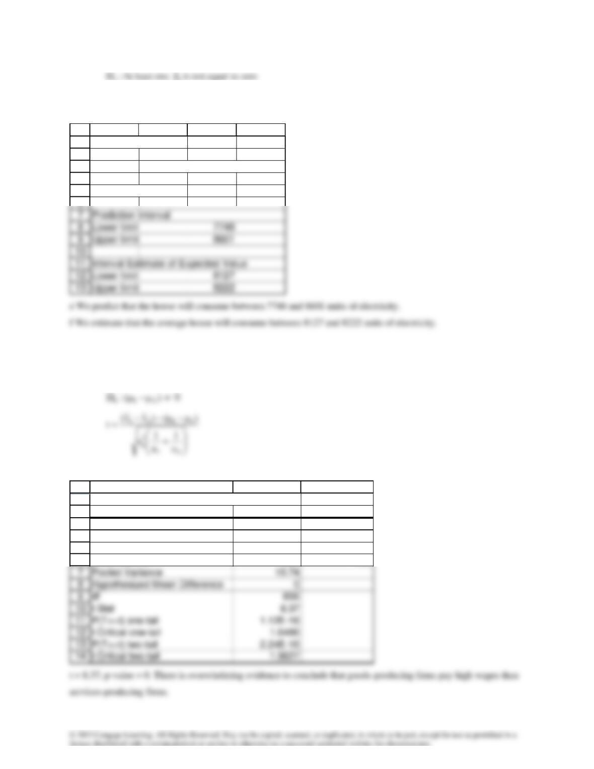
F = 117.6, p-value = 0. There is enough evidence to conclude that the model is valid.
d & e
1
2
3
4
5
A B C D
Prediction Interval
Consumption
Predicted value 8175
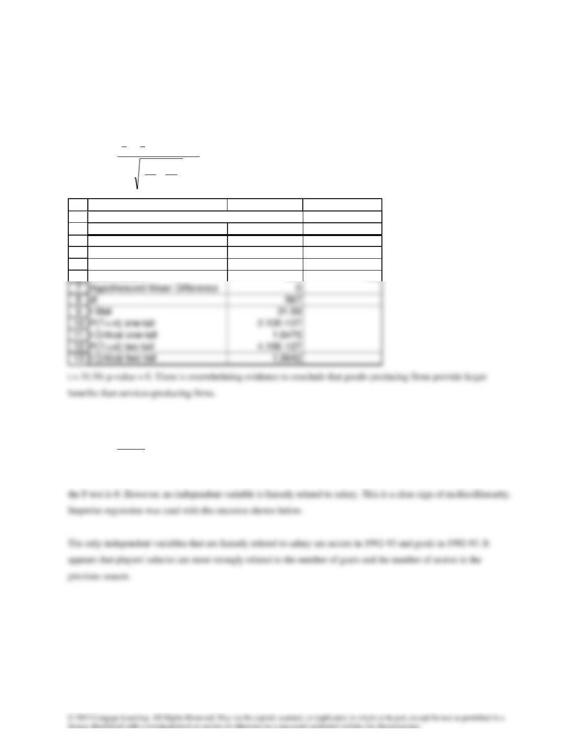
A17.13Wages: Equal-variances t-test of
21 −
)(:H 210 −
= 0
1
2
3
4
5
6
A B C
t-Test: Two-Sample Assuming Equal Variances
Goods wages Service wages
Mean 18.66 16.78
Variance 11.54 10.05
Observations 395 463
Benefits: Unequal-variances t-test of
21 −
)(:H 210 −
= 0
)(:H 211 −
0
+
−−−
=
2
2
2
1
2
1
2121
n
s
n
s
)()xx(
t
1
2
3
4
5
6
A B C
t-Test: Two-Sample Assuming Unequal Variances
Goods benefits Service benefits
Mean 9.82 6.34
Variance 3.91 1.03
Observations 395 463
A17.14 Multiple regression, test of coefficients
i
b
ii
s
b
t−
=
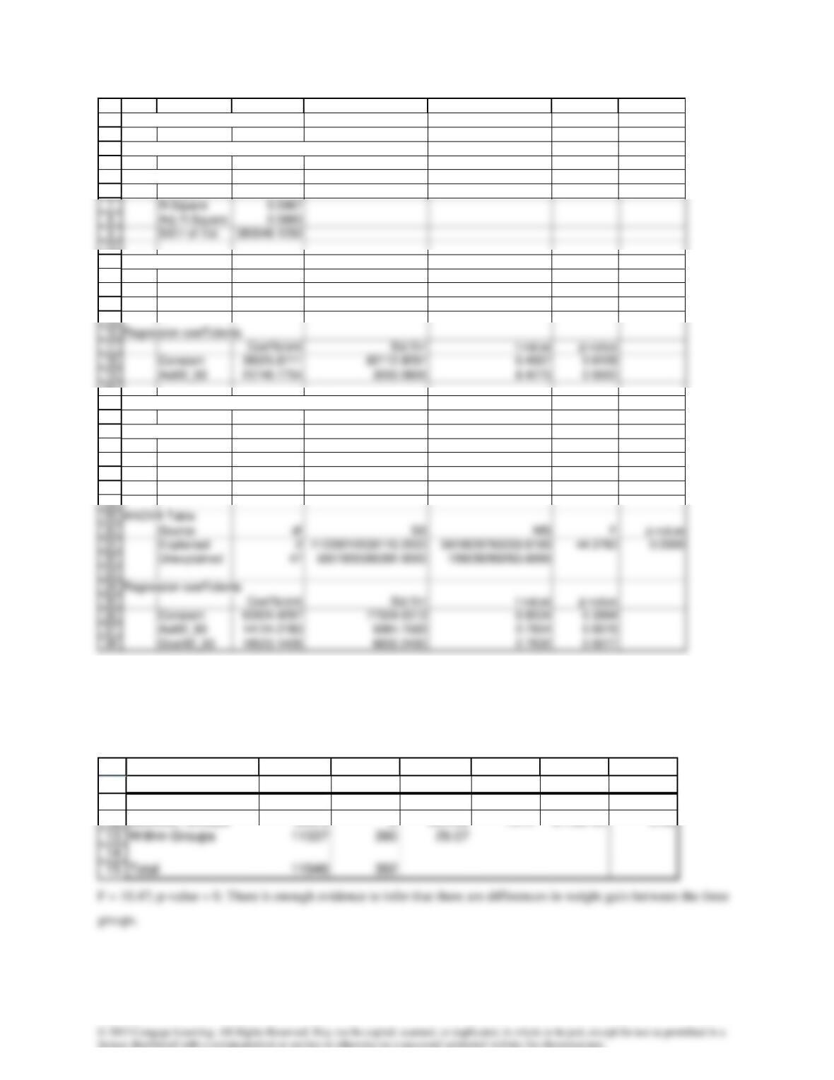
The ordinary multiple regression model fit quite well. The coefficient of determination is .7042 and the p–value of
1
2
3
4
5
6
10
11
12
13
14
20
21
22
23
24
25
26
27
M N O P Q R S
Results of stepwise regression
Step 1 – Entering variable: Ast92_93
Summary measures
Multiple R 0.7725
ANOVA Table
Source df SS MS F p-value
Explained 1 10258242603399.2000 10258242603399.2000 71.0232 0.0000
Unexplained 48 6932882522112.0000 144435052544.0000
Step 2 – Entering variable: Goal92_93
Summary measures Change % Change
Multiple R 0.8086 0.0361 %4.7
R-Square 0.6538 0.0571 %9.6
Adj R-Square 0.6390 0.0507 %8.6
StErr of Est 355859.9375 -24186.1875 -%6.4
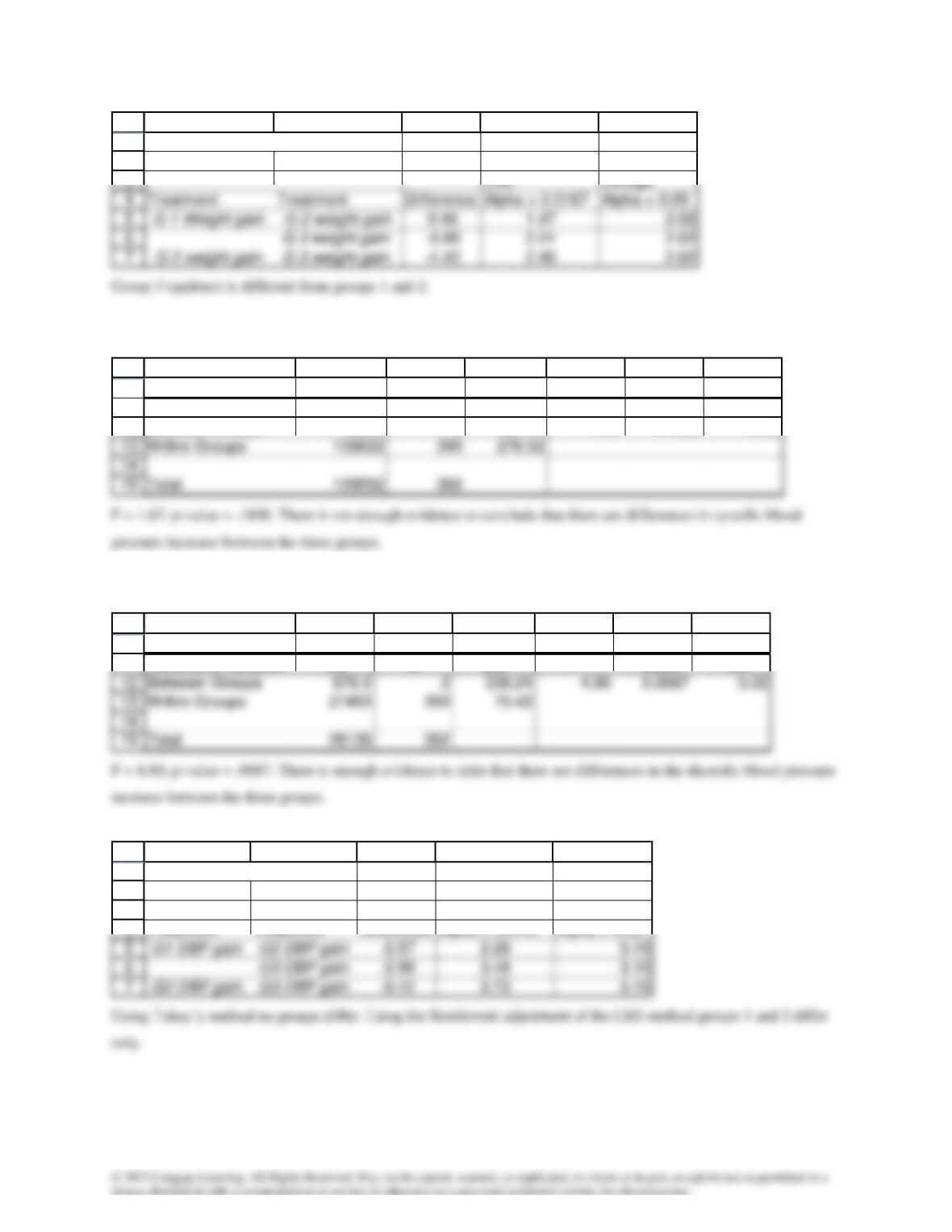
A17.15One-way analysis of variance
3210 :H ==
Weight gain
10
15
11
12
A B C D E F G
ANOVA
Source of Variation SS df MS F P-value F crit
Between Groups 608.6 2 304.32 10.47 3.73E-05 3.02
1
2
A B C D E
Multiple Comparisons
Systolic blood pressure increase
10
15
11
12
A B C D E F G
ANOVA
Source of Variation SS df MS F P-value F crit
Between Groups 929.6 2 464.78 1.67 0.1898 3.02
Diastolic blood pressure increase
10
12
15
Between Groups 676.5 2 338.24 4.80 0.0087 3.02
11
A B C D E F G
ANOVA
Source of Variation SS df MS F P-value F crit
1
2
3
A B C D E
Multiple Comparisons
LSD Omega
A17.16 t-estimator of µ