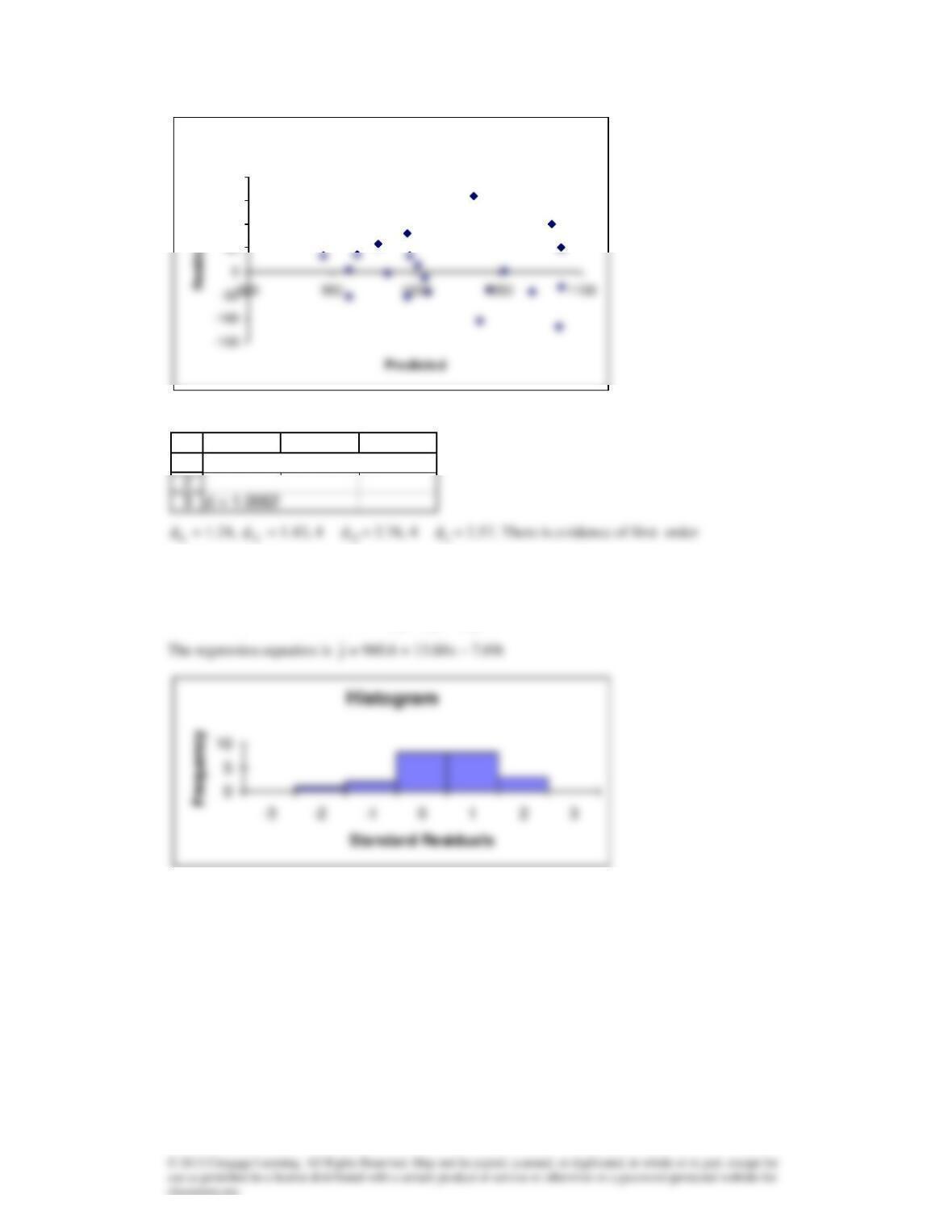
The normality requirement is satisfied. However, the constant variance requirement is not.
autocorrelation.
c The problem is that the errors are not independent. We add a time variable (week number) to the
model. Thus, the new model is y =
0
+
x
1
+
t
2
+
.
Plot of Residuals vs Predicted
50
100
150
200
1
A B C
Durbin-Watson Statistic
L
U
U
L
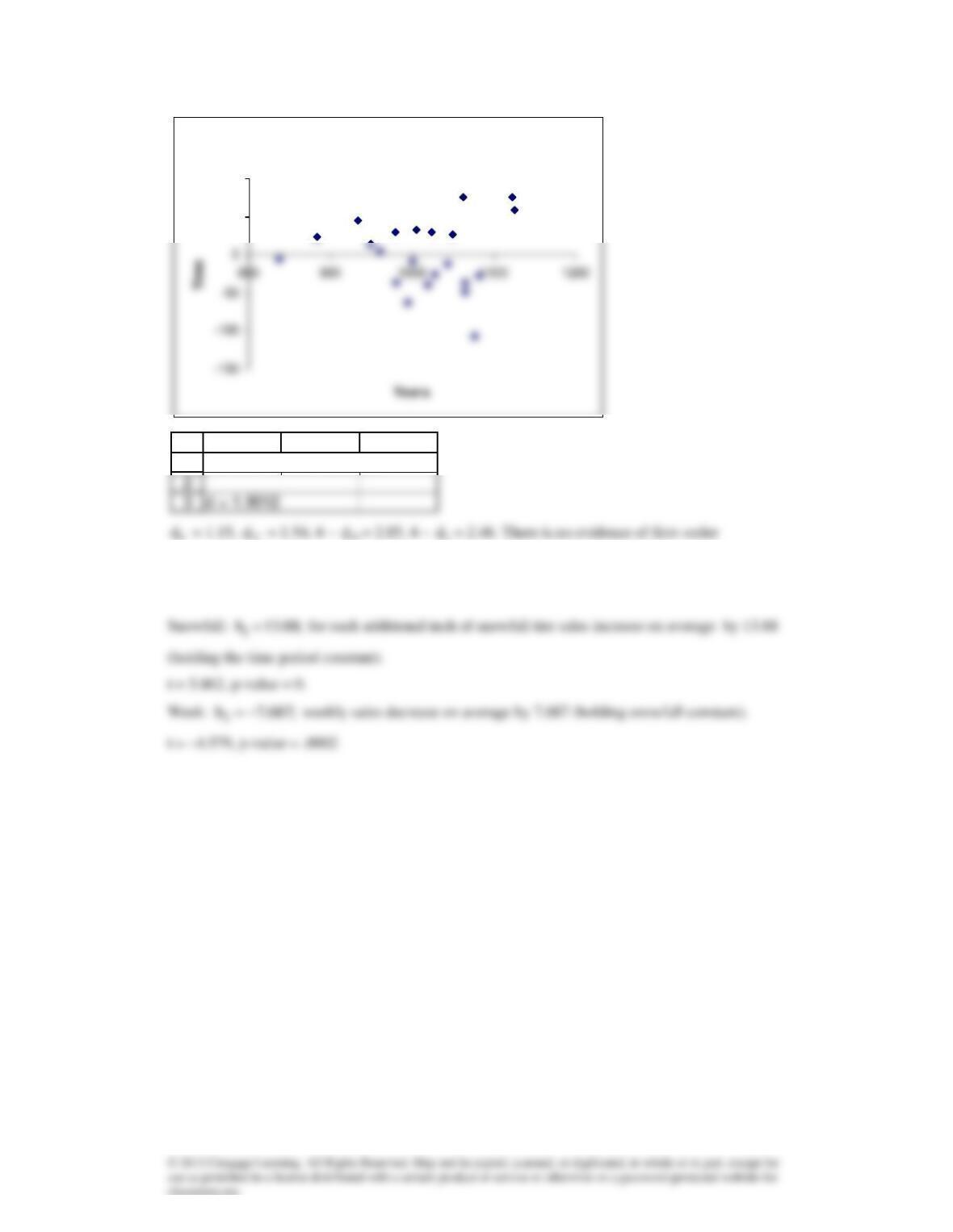
autocorrelation.
d
s
= 48.55 and
2
R
= .7040
Plot of Residuals vs Years
50
100
1
A B C
Durbin-Watson Statistic

17.54a
21 x0313.x140.01.164y
For each additional unit of fertilizer crop yield increases on average by .140 (holding the amount
of water constant).
For each additional unit of water crop yield increases on average by .0313 (holding the fertilizer
constant).
b
:H0
=1
0
0:H 11
:H0
1
2
3
4
5
6
A B C D E F
SUMMARY OUTPUT
Regression Statistics
Multiple R 0.6894
R Square 0.4752
Adjusted R Square 0.4363
e
f
10
20
Histogram
50
100
150
Plot of Residuals vs Predicted
1
2
3
4
5
A B
Prediction Interval
Yield
Predicted value 209.3

17.55
21
b
:H0
=1
0
432 ===
:H1
At least one
i
is not equal to zero
1
2
8
3
4
9
10
14
11
12
15
16
17
A B C D E F
SUMMARY OUTPUT
Regression Statistics
Multiple R 0.6882
ANOVA
df SS MS F Significance F
Regression 4 220,130,124 55,032,531 7.87 0.0001
Coefficients Standard Error t Stat P-value
Intercept 1,433 2,093 0.68 0.4980
14
15
19
b
;6123.R2=
61.23 % of the variation in rents is explained by the independent variables.
:H0
:H1
i
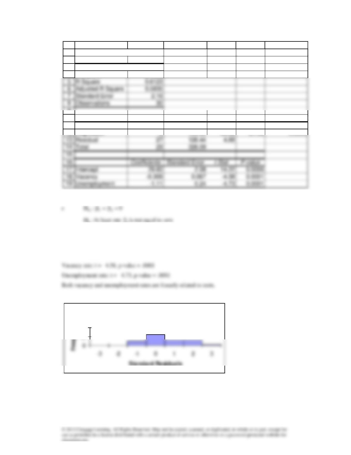
F = 21.32, p-value = 0. There is enough evidence to conclude that the model is valid.
d
:H0
=i
0
:H1
i
0
e
1
2
8
3
4
9
10
11
12
A B C D E F
SUMMARY OUTPUT
Regression Statistics
Multiple R 0.7825
ANOVA
df SS MS F Significance F
Regression 2 199.65 99.82 21.32 0.0000
Histogram
10
20
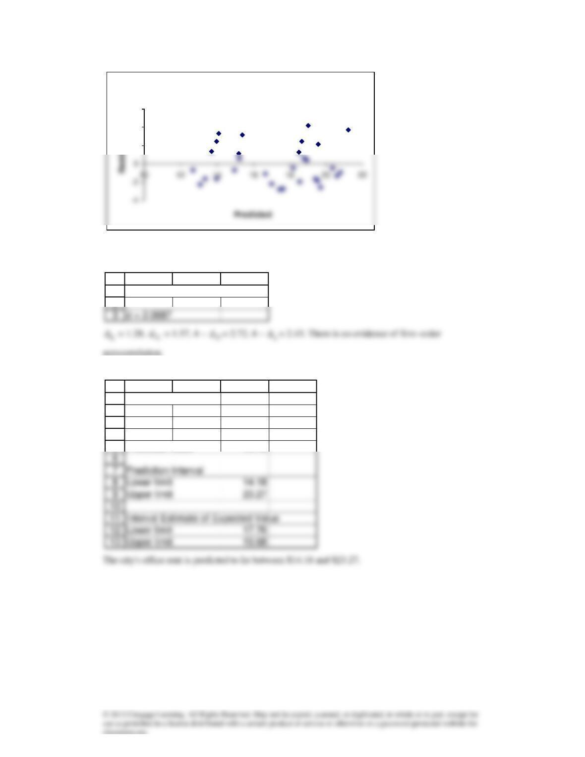
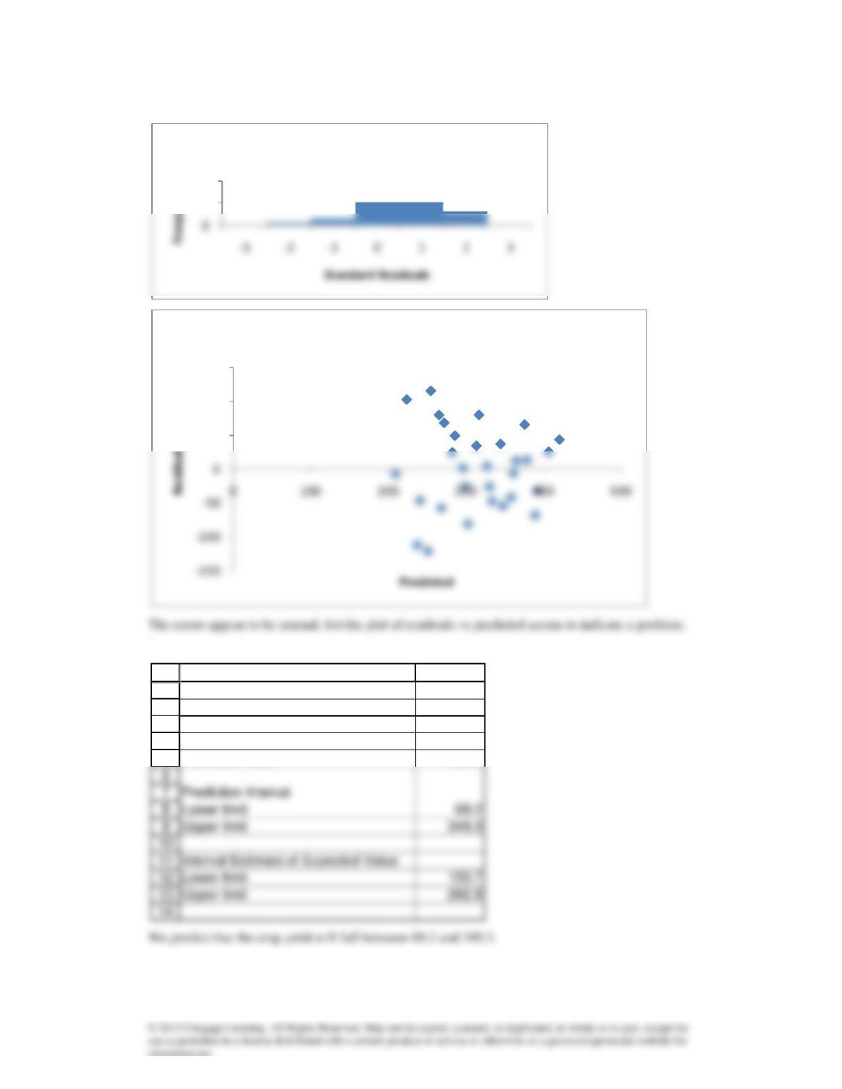
The error is approximately normally distributed with a constant variance.
f
autocorrelation.
g
Plot of Residuals vs Predicted
2
4
6
1
2
A B C
Durbin-Watson Statistic
1
2
3
4
5
A B C D
Prediction Interval
Rent
Predicted value 18.72

Case 17.1
14
The model is valid (F = 7.75, p-value = 0) but the model does not fit well (R
2
= .0151; only 1.51%
of the variation in returns is explained by the model).
Interpreting the coefficients in this sample:
For each additional one–point increase in the SAT score, returns increase on average by .0051
Testing the coefficients:
SAT: t = 3.96, p-value = .0001
1
2
8
3
9
10
11
12
13
A B C D E F
SUMMARY OUTPUT
Regression Statistics
ANOVA
df SS MS F Significance F
Regression 4 2,137 534.29 7.75 0.0000
Residual 2024 139,561 68.95

There is overwhelming evidence to infer that SAT scores of the undergraduate university and age
Case 17.2
Analysis of Betas
Interpreting the coefficients in this sample:
For each additional one–point increase in the SAT score, betas increase on average by .00050
provided the other variables remain constant.
1
2
3
4
9
10
11
12
A B C D E F
SUMMARY OUTPUT
Regression Statistics
Multiple R 0.3597
ANOVA
df SS MS F Significance F
Regression 4 15.15 3.79 75.20 0.0000

Testing the coefficients:
SAT: t = 14.55, p-value = 0
There is overwhelming evidence to infer that all four independent variables are linearly related to
mutual fund betas.
Analysis of MERs
22
Interpreting the coefficients in this sample:
For each additional one–point increase in the SAT score, MERs decrease on average by .00055
provided the other variables remain constant.
1
2
8
10
14
3
4
5
15
16
17
18
19
A B C D E F
SUMMARY OUTPUT
Regression Statistics
Multiple R 0.2697
R Square 0.0728
Coefficients Standard Error t Stat P-value
Intercept 2.89 0.183 15.73 0.0000
SAT -0.00055 0.00011 -5.21 0.0000
MBA -0.082 0.0310 -2.65 0.0081
For each additional one–year increase in the manager’s job tenure, MERs increase on average by
.0375 provided the other variables remain constant.
For each additional one–point increase in the log of the assets, MERs decrease on average by .209
provided the other variables remain constant.