
CHAPTER 1
The problems in this chapter are of two general types: (1) those that focus on
intertemporal maximization and (2) those that ask students to make fairly simple present
discounted value calculations. Before undertaking any of these, students should be sure to read
the Appendix in Chapter 17. The appendix is especially important for problems involving
continuous compounding because students may not have encountered that concept in earlier
courses.
Comments on Problems
17.1 This problem is a simple analysis of intertemporal choices. The problem illustrates the
indeterminacy of the sign of the effect of the real interest rate on current savings. Part (c)
concerns intertemporal allocation with initial endowments in both periods.
17.2 This is a present discounted value problem. I have found that the problem is most easily
solved using continuous compounding (see below), but the discrete approach is also
relatively simple. Instructors may wish to point out that the savings rate calculated here
(22.5%) is considerably above the personal savings rate in the United States.
17.3 This is a simple present discounted value problem that should be solved with continuous
compounding.
17.4 This is a traditional capital theory problem involving trees. Students seem to have
difficulty in seeing their way through this problem and in interpreting the results. Hence,
instructors may wish to allow some time for discussion of it.
17.5 This problem is a discussion question that asks students to explore the logic of the U.S.
corporate income tax. The case of accelerated depreciation is, I believe, a particularly
effective example of the time value of money.
17.6 This problem presents a discounted value example of life insurance sales tactics. Students
tend to like this problem and, I’m told, some have even used its results when approached
by actual salespeople.
CHAPTER 17:
Capital and Time

Chapter 17: Capital and Time
196
17.7 This problem is a simple numerical example of the “Hotelling rule” for natural resource
pricing developed in the text.
Analytical Problems
17.8 Capital gains taxation. This is a graphic problem that shows how changes in the interest
rate induce capital gains that might be taxed.
17.9 Precautionary saving and prudence. This is a simple example showing how uncertainty
can be incorporated into the saving model presented in the chapter. It shows that the third
derivative of the utility function matters.
17.10 Monopoly and natural resource prices. This is a resource economics problem that
shows, with a finite resource, monopoly pricing options are severely constrained.
17.11 Renewable timber economics. This is a continuation of Problem 17.4, which shows that
optimal timber harvesting rules may be a bit different once the possibility of replanting is
considered.
17.12 More on the rate of return on a risky asset. This problem pursues the asset pricing
material in the chapter with a more explicit focus on the expected rate of return. It
describes the Sharpe ratio and uses the bound on that ratio to provide a simple example of
the equity premium puzzle.
17.13 Hyperbolic discounting. This behavioral problem introduces Laibson’s hyperbolic
utility function and provides a relatively intuitive presentation of the intertemporal
behavior implied by this function.
Solutions
17.1
a. The Lagrangian expression for this maximization problem is
Chapter 17: Capital and Time
197
Division of the first two of these yields
c. Budget constraint has same slope as in part (a) and passes through the point
17.2 This problem can be most easily worked using continuous time:
Accumulated savings after 40 years
Present value of spending in retirement
For accumulated savings to equal the present value of dissavings, it must be the
case that
17.3 Using Equation 17.55 yields
Chapter 17: Capital and Time
198
17.4
a. The present value of the wood in any tree is given by
()
rt
e f t
−
. As before, to
c, d. The total value of a balanced woodlot is found by integration over all vintages of
trees:
c. Tend to increase use of capital since there is a tax advantage in early years. Total
Chapter 17: Capital and Time
199
17.6 For the whole life policy, the present value of premiums paid is
17.7 Using Equation 17.71, we get
Analytical Problems
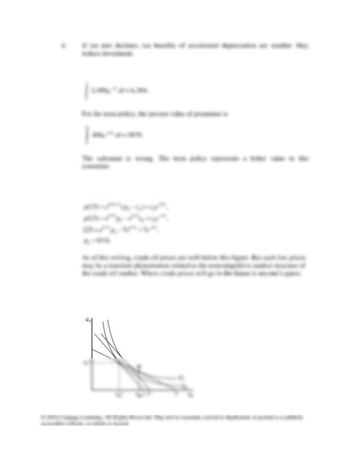
17.8 Capital gains taxation
Chapter 17: Capital and Time
200
d. Realized capital gains are given by distance
*
0,B
cc
that is the present value of one-
period bonds that must be sold to attain the new utility-maximizing choice of cB.
17.9 Precautionary saving and prudence
a. In the context of uncertainty, the person will aim to maximize the total expected
utility. Thus, if consumption is certain in the current period and uncertain in the
b. If
U
is convex, Jensen’s inequality gives
U
[ ( )] ‘[ ( ].E U c U E c
U
c. The person with convex
U
will opt for a higher scheduled level of consumption
Chapter 17: Capital and Time
201
d. The above considerations imply that a faster consumption growth rate is optimal
17.10 Monopoly and natural resource prices
a. If the resource is owned by a single firm, then the firm sets the market price.
b. The Hamiltonian would be
The first of these conditions can be simplified as
=− −rt
etctMR )]()([
.
Differentiation with respect to t yields
c. This equation implies almost identical price dynamics as under competition. For
17.11 Renewable timber economics
Chapter 17: Capital and Time
202
So, for a maximum,
c. The condition implies that, at optimal
*
t
, the increased wood obtainable from
17.12 More on the rate of return on a risky asset
b. This is just a direct application of the Cauchy–Schwartz inequality to the equation
derived in part (a). One way to see why the Cauchy–Schwartz inequality holds is
Chapter 17: Capital and Time
203
e. The Sharpe ratio for common stocks is about 0.5—the long-run real rate of return
17.13 Hyperbolic discounting
a. For the given utility function, the discount factors have the following values:
b. The significant drop of the discount factors for period t + 1 means that preferences
c. In period t, the MRS between ct+1 and ct+2 will be
).(/)( 21 ++ tt cUcU
d. Constraints are necessary so as to avoid changes in the consumption decision

Chapter 17: Capital and Time
204
e. Examples include retirement funds with penalties for early withdrawal of funds,
a form of commitment against future overconsumption.