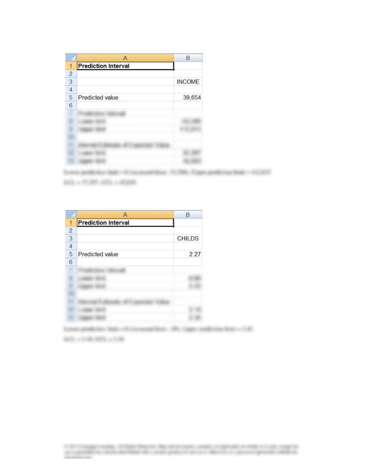
16.95
16.96
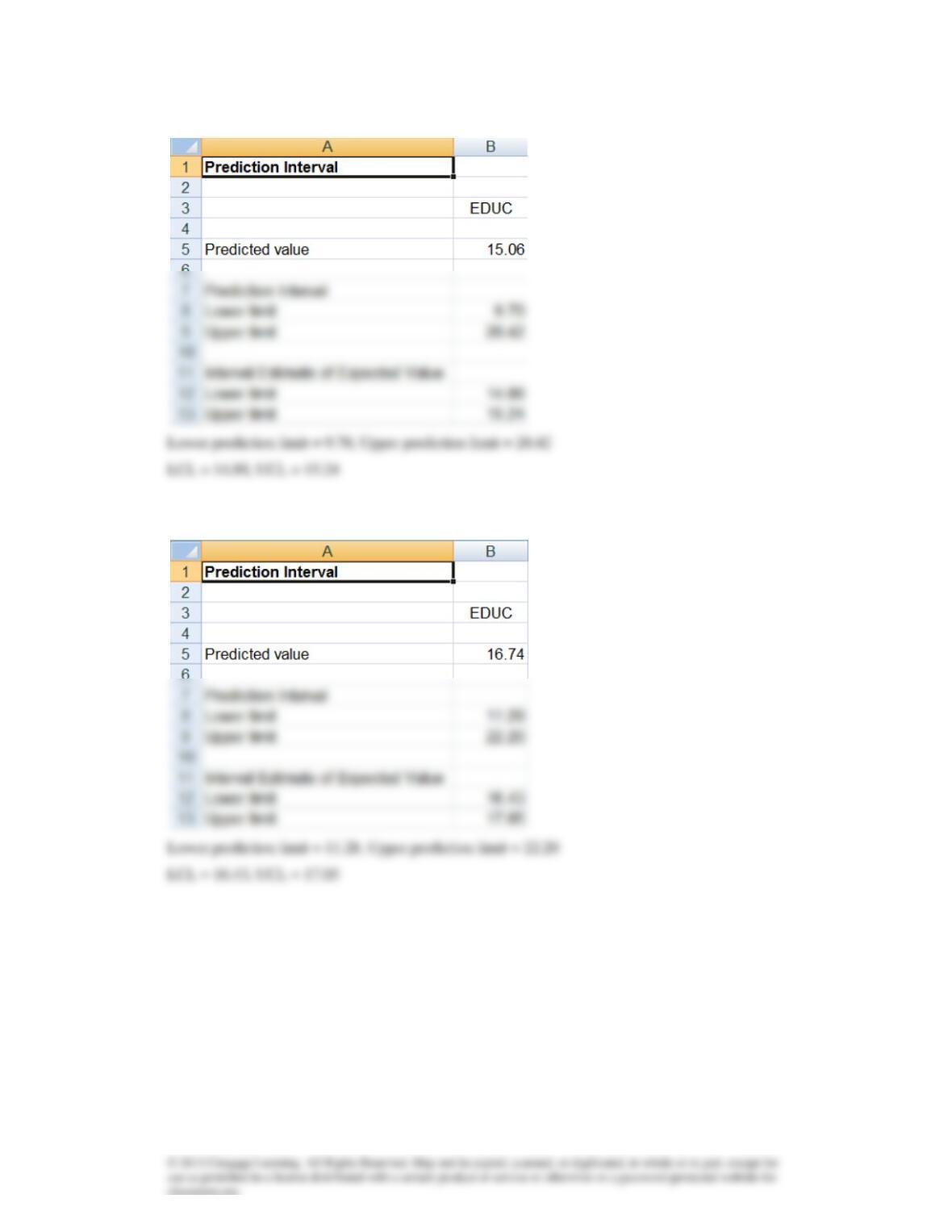
16.97
16.98
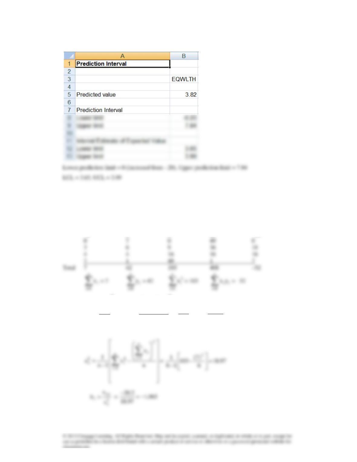
16.99
16.100 In all cases the linear relationship is far too weak to produce accurate predictions.
16.101 a
i
x
i
y
2
i
x
2
i
y
iiyx
–5 15 25 225 –75
–2 9 4 81 –18
−
−
=
==
=n
yx
yx
1n
1
s
n
1i
i
n
1i
i
n
1i
iixy
=
20.20
6
42)(7(
52
16
1−=
−−
−
The sample regression line is
y
ˆ
= 8.253 – 1.065x
b, c, &d
−
−
=
=
=n
y
y
1n
1
s
2
n
1i
i
n
1i
2
i
2
y
=
80.22
6
)42(
408
16
12
=
−
−
i
x
i
y
x065.1253.8y
ˆi−=
iii y
ˆ
ye −=
s/ei
–5 15 13.58 1.42 1.118
–2 9 10.38 –1.38 –1.087
0 7 8.253 –1.253 –.987
16.102
i
x
i
y
x0582.107.9y
ˆi−=
iii y
ˆ
ye −=
23 9.6 10.45 –.85
46 11.3 11.78 –.48
60 12.8 12.60 .20
16.103
i
i
iii y
x
y
y
ˆ
= 475.2 – 39.17x
ˆ
ye −=
7.6 185 177.5 7.5
7.5 201 181.4 19.6
8.0 206 161.8 44.2
16.104 a & b
i
x
i
y
y
ˆ
= – 24.72 + .9675x
iii y
ˆ
ye −=
42 18 15.92 2.09
34 6 8.18 –2.18
25 0 –.53 .53
35 –1 9.14 –10.14
c
16.105
i
x
i
y
y
ˆ
= –100,652 + 1,513x
iii y
ˆ
ye −=
80 20,533 20,388 145
68 1,439 2,232 –793
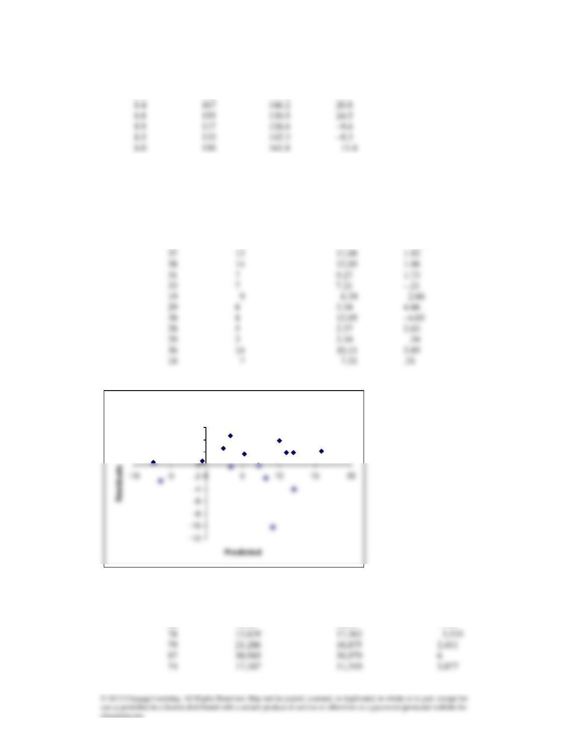
Plot of Residuals vs Predicted
2
4
6
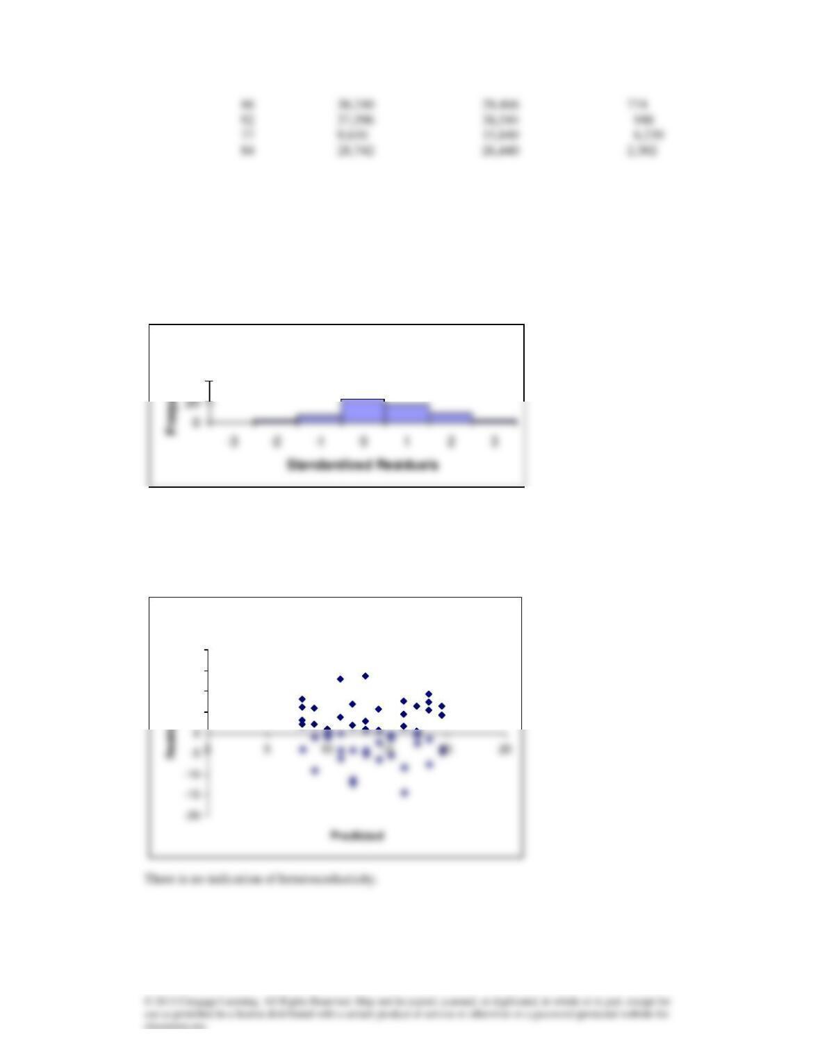
The histograms drawn below are of the standardized residuals, which make it easier to see
whether the shape is extremely nonnormal. It also makes it easier to identify outliers. The shape of
the resulting histogram is identical to the histogram of the residuals using the equivalent class
limits.
16.106 b & c
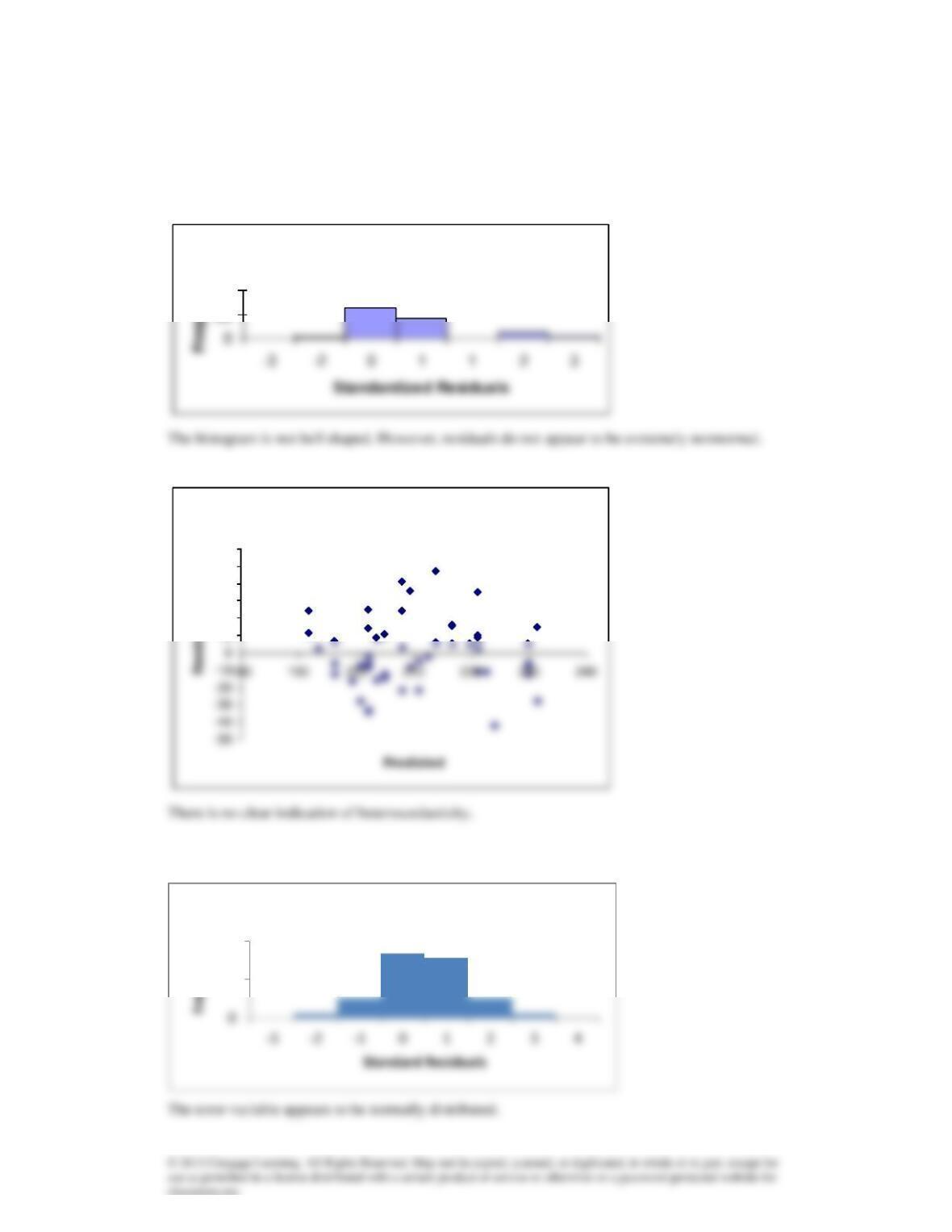
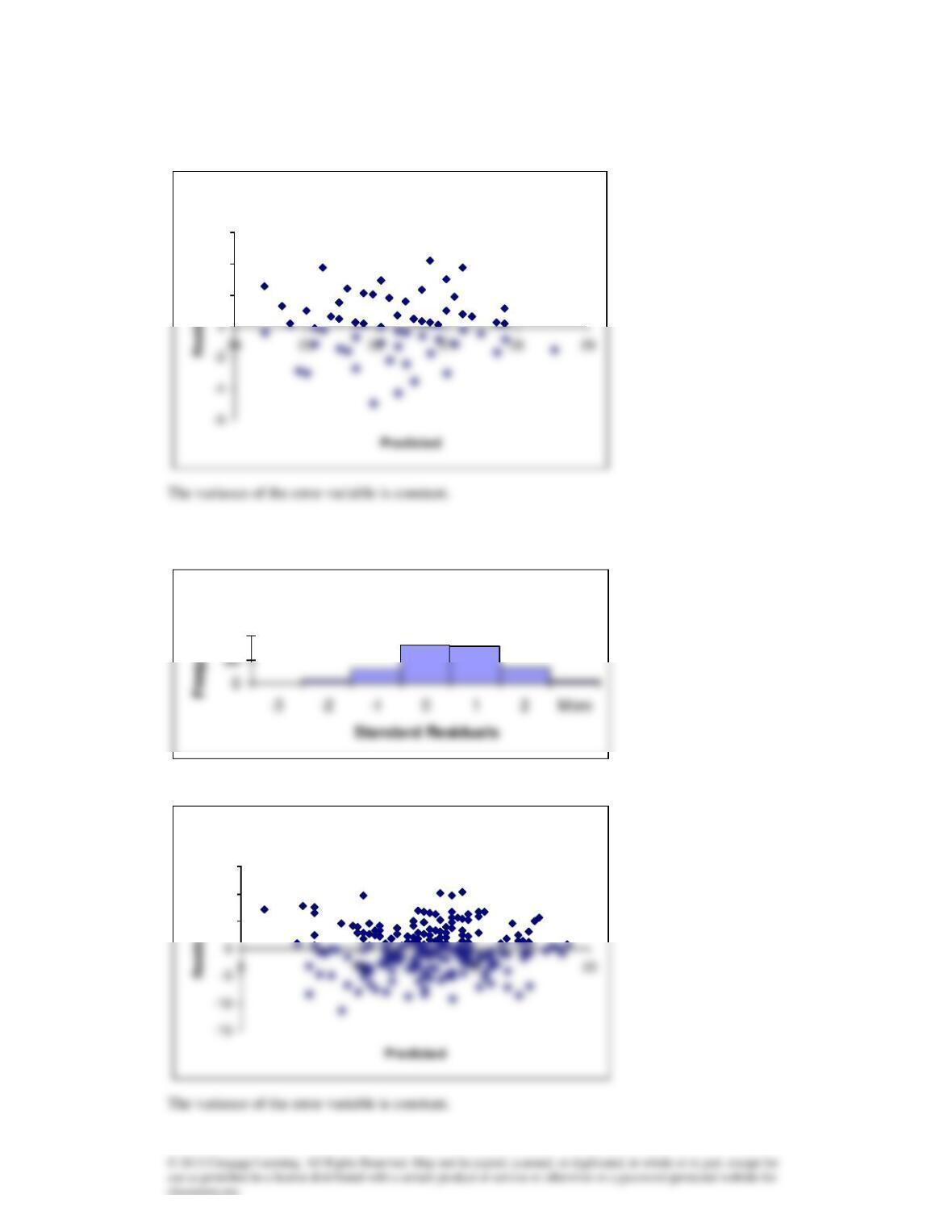
Because the histogram is approximately bell shaped the errors appear to be normally distributed.
There are two residuals whose absolute value exceeds 2.0.
d
Histogram
40
Plot of Residuals vs Predicted
5
10
15
20
16.107 a
c
16.108
Histogram
20
40
Plot of Residuals vs Predicted
10
20
30
40
50
60
50
100
Histogram
16.109 b & c
10
15
20
25
Plot of Residuals versus Predicted
Histogram
20
40
d
16.110
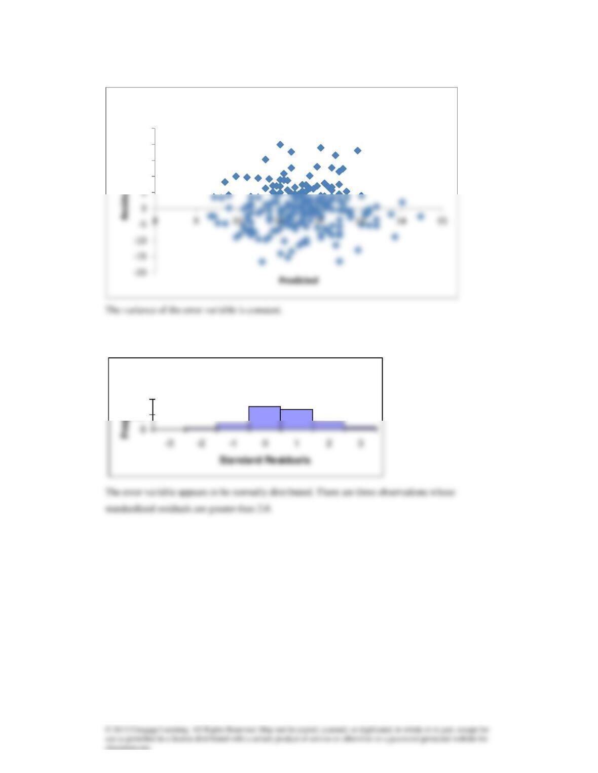
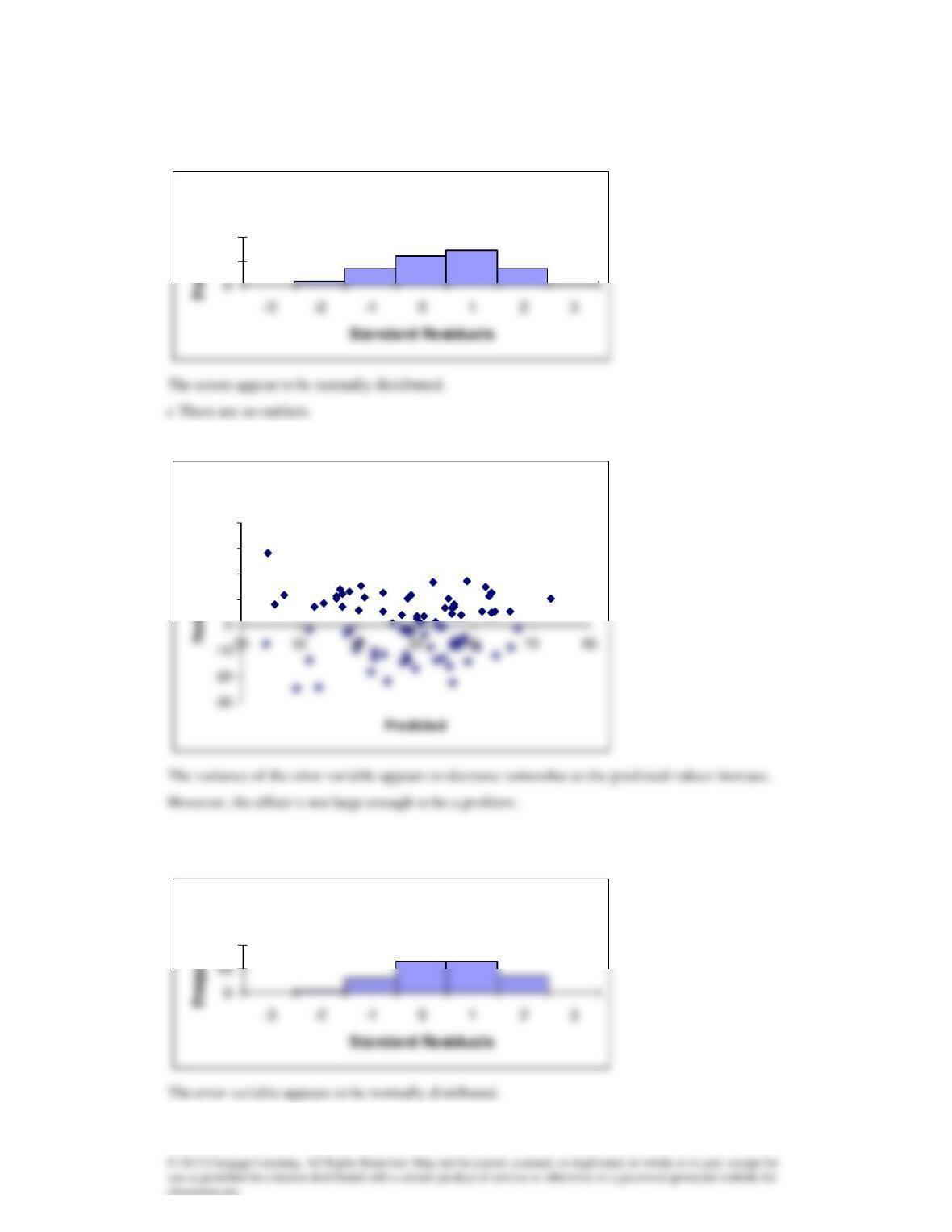
The error variable appears to be normally distributed.
Plot of Residuals vs Predicted
2
4
6
Histogram
100
Plot of Residuals vs Predicted
5
10
15
16.111b
d
16.112
10
Histogram
20
40
Plot of Residuals vs Predicted
10
20
30
40
Histogram
20
16.113
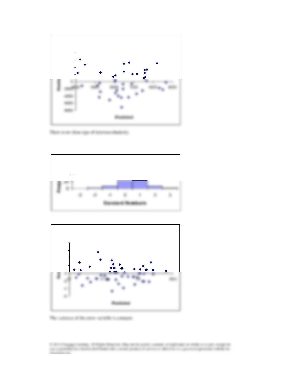
The error variable appears to be normally distributed.
Plot of Residuals vs Predicted
2000
4000
6000
8000
Histogram
40
Plot of Residuals vs Predicted
2
4
6
8
16.114
16.115
100
Histogram
200
400
600
Plot of Residuals vs Predicted
Histogram
50
100