Chapter 16
16.1 a The slope coefficient tells us that for additional inch of father’s height the son’s height
16.2 a
b
i
x
i
y
2
i
x
2
i
y
iiyx
23 9.6 529 92.16 220.8
46 11.3 2,116 127.69 519.8
60 12.8 3,600 163.84 768.0
54 9.8 2,916 96.04 529.2
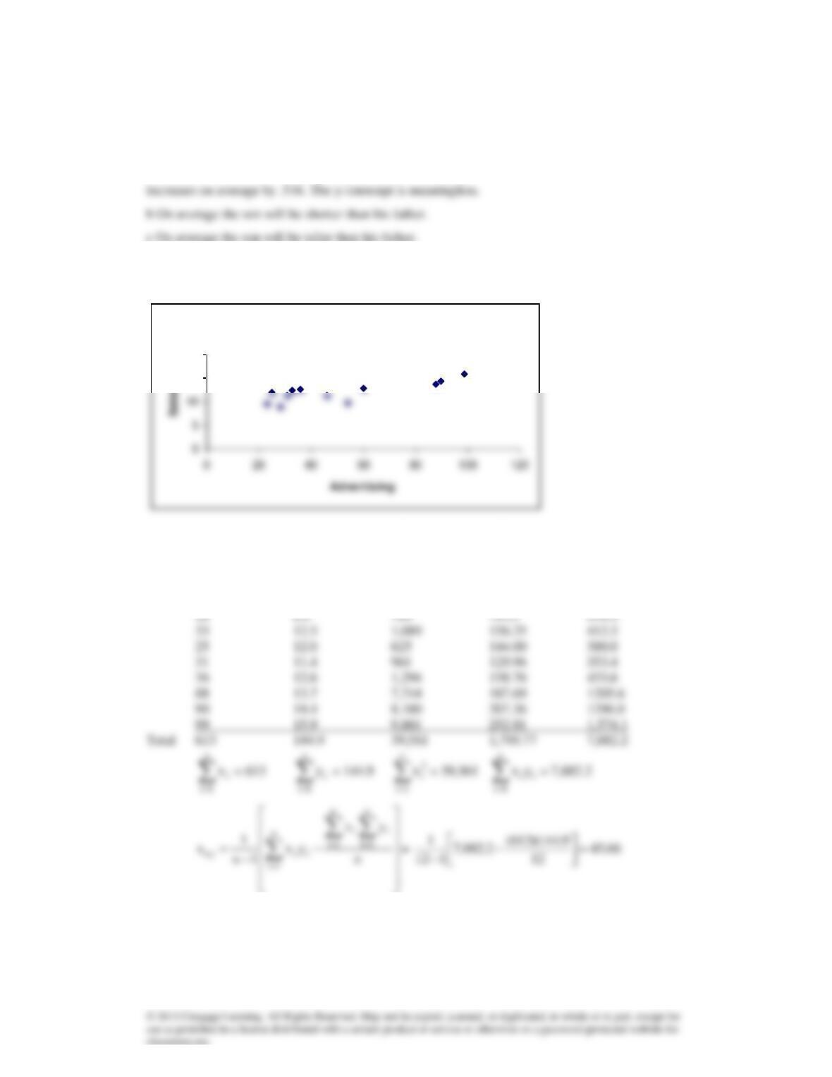
Scatter Diagram
15
20
−
−
=
=
=n
x
x
1n
1
s
2
n
1i
i
n
1i
2
i
2
x
=
7.749
12
)613(
561,39
112
12
=
−
−
The sample regression line is
y
ˆ
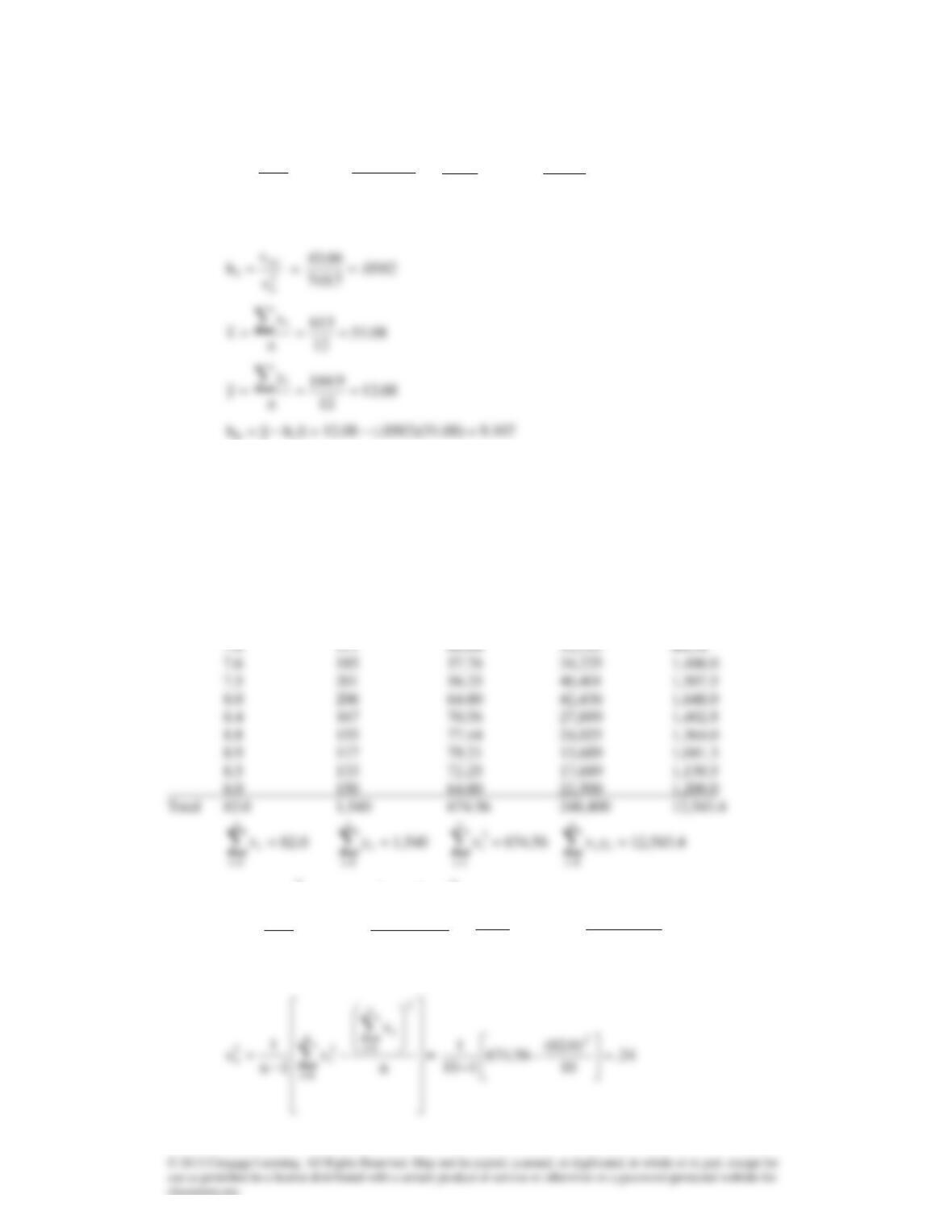
= 9.107 + .0582x
The slope tells us that for each additional thousand dollars of advertising sales increase on average
by .0582 million. The y-intercept has no practical meaning.
16.3 a
i
x
i
y
2
i
x
2
i
y
iiyx
8.5 115 72.25 13,225 977.5
−
−
=
==
=n
yx
yx
1n
1
s
n
1i
i
n
1i
i
n
1i
iixy
=
40.9
10
540,1)(0.82(
4.543,12
110
1−=
−
−
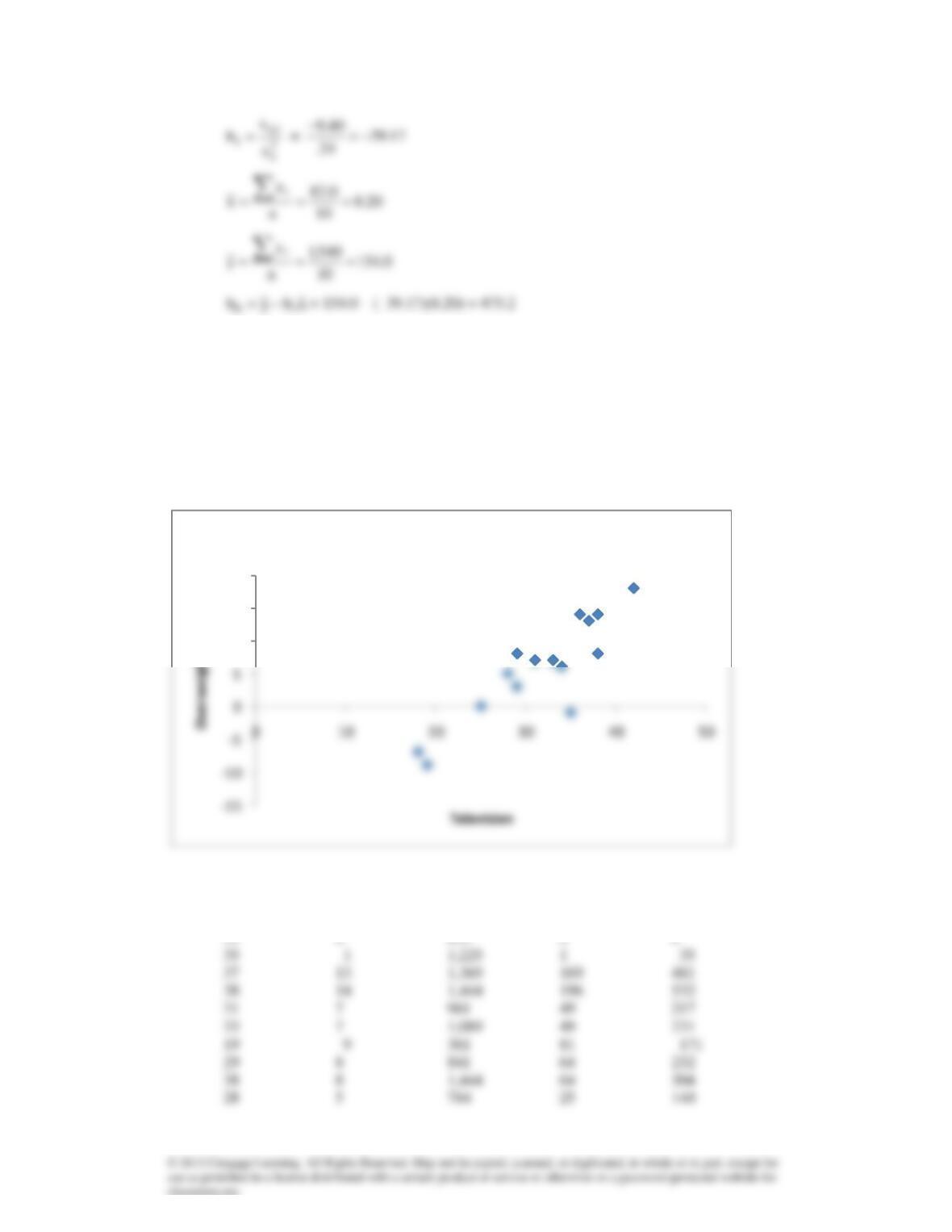
The sample regression line is
y
ˆ
= 475.2 – 39.17x
b. The slope coefficient tells us that for each additional 1 percentage point increase in mortgage
rates, the number of housing starts decreases on average by 39.17. The y-intercept has no
meaning.
16.4a
b
i
x
i
y
2
i
x
2
i
y
iiyx
42 18 1,764 324 756
34 6 1,156 36 204
25 0 625 0 0
10
15
20
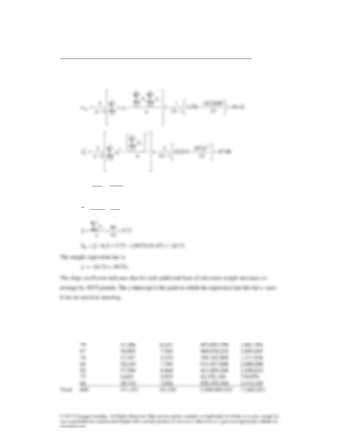
Scatter Diagram
29 3 841 9 87
36 14 1,296 196 504
18 –7 324 49 –126
Total 472 86 15,524 1,312 3,356
=
n
1i
i
x
= 472
=
n
1i
i
y
= 86
=
n
1i
2
i
x
= 15,524
=
n
1i
ii yx
= 3,356
2
x
xy
1s
s
b=
=
9675.
98.47
42.46 =
47.31
15
472
n
x
xi===
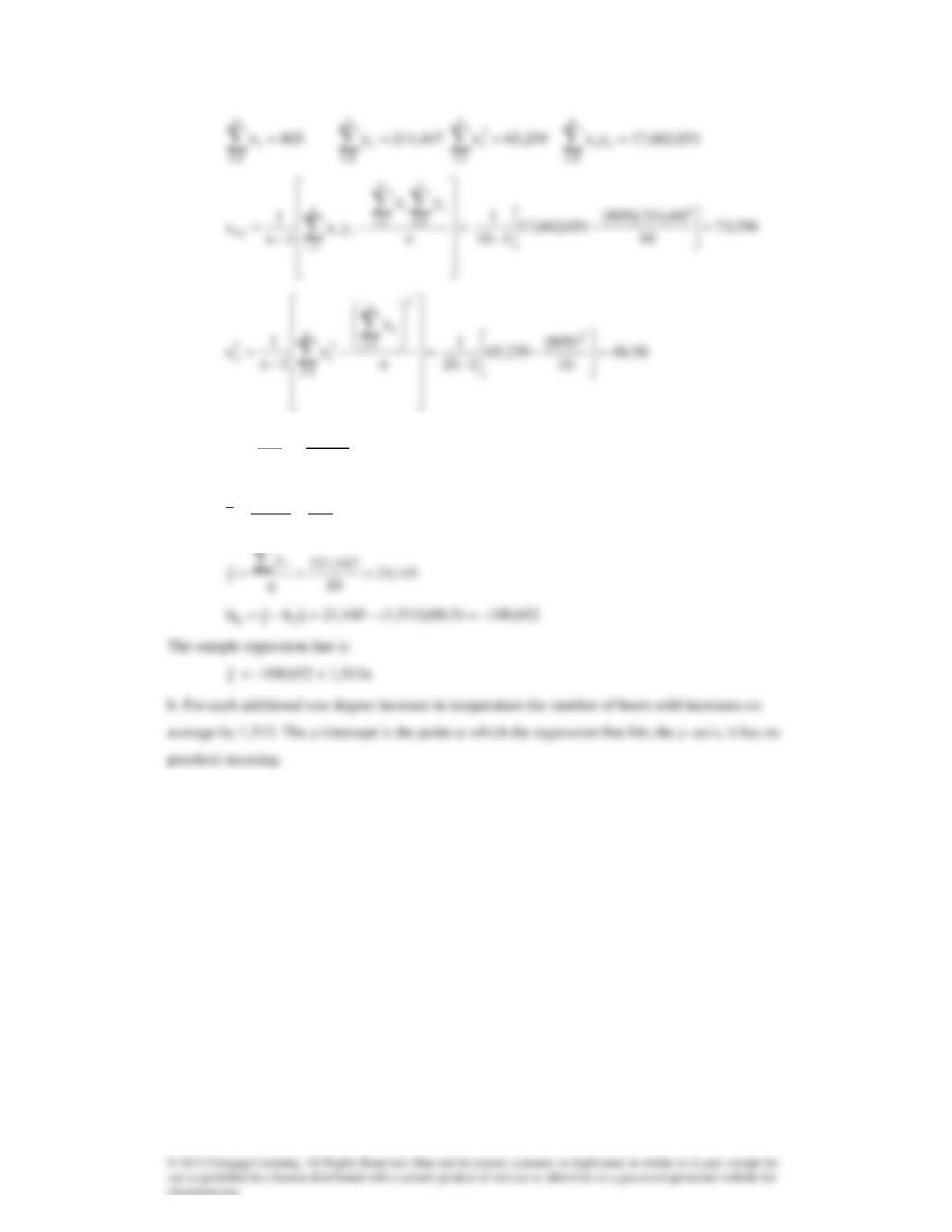
16.5a
i
x
i
y
2
i
x
2
i
y
iiyx
80 20,533 6,400 421,604,089 1,642,640
68 1,439 4,624 2,070,721 97,852
78 13,829 6,084 191,241,241 1,078,662
2
x
xy
1s
s
b=
=
513,1
50.48
396,73 =
5.80
10
805
n
x
xi===
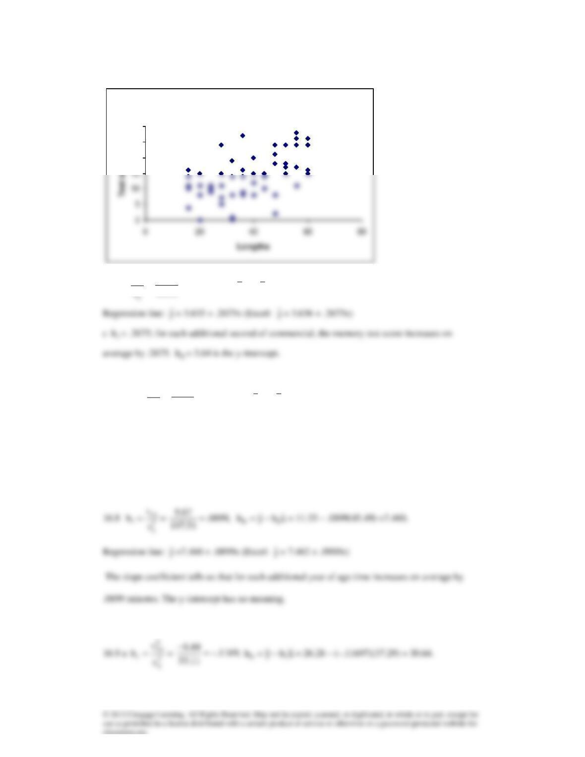
16.6 a
b
x
y
ˆ
y
ˆ
2
xy
1s
s
b=
=
9.193
86.51
= .2675,
xbyb 10 −=
= 13.80 – .2675(38.00) = 3.635
16.7a
2
x
xy
1s
s
b=
=
,465.1
32.59
93.86 =
xbyb 10 −=
= 210.4 – 1.465(13.68) =190.4.
Regression line:
y
ˆ
= 190.4 + 1.465x (Excel:
y
ˆ
= 190.4 + 1.465x)
b For each additional floor prices increase on average by $1.465 thousand ($1,465). The y–
intercept has no practical meaning.
2
x
xy
1s
s
b=
xbyb 10 −=
y
ˆ
y
ˆ
xbyb 10 −=
Scatter Diagram
20
25
30
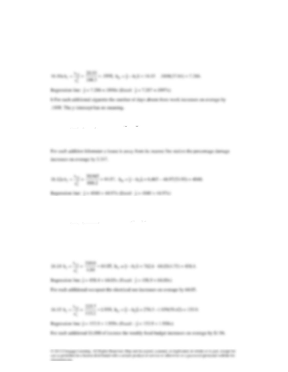
Regression line:
y
ˆ
= 30.64 – .1169x (Excel:
y
ˆ
= 30.63 – .1169x)
b The slope coefficient indicates that for each additional year of age, the employment period
decreases on average by .1169.
0
b
= 30.63 is the y-intercept.
2
x
xy
1s
s
b=
y
ˆ
y
ˆ
16.11
2
x
xy
1s
s
b=
=
,347.5
270.4
83.22 =
xbyb 10 −=
= 49.22 – 5.347(4.885) = 23.10.
Regression line:
y
ˆ
= 23.10 + 5.347x (Excel:
y
ˆ
= 23.11 + 5.347x)
2
x
xy
1s
s
b=
y
ˆ
y
ˆ
b. For each additional thousand square feet the price increases on average by $44.97 thousand.
16.13
2
x
xy
1s
s
b=
=
,00138.
153,59
78.81 −=
−
xbyb 10 −=
= 27.73 – (–.00138)(1199) = 29.39.
Regression line:
y
ˆ
= 29.39–.00138x (Excel: 29.39–.00138x)
For each additional hour the price decreases on average by .00138 thousand dollars or $1.38.
2
x
xy
1s
s
b=
xbyb 10 −=
y
ˆ
y
ˆ
2
x
xy
1s
s
b=
xbyb 10 −=
y
ˆ
y
ˆ
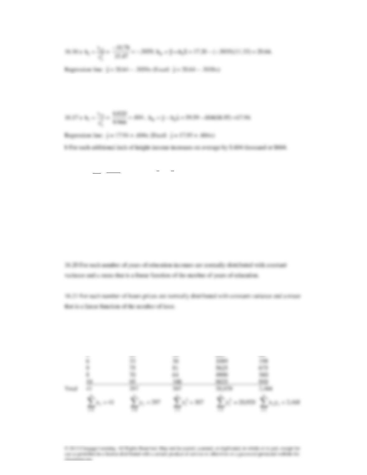
b The slope indicates that for each additional one percentage point increase in the vacancy rate
rents on average decrease by $.3039.
y
ˆ
y
ˆ
16.18
2
x
xy
1s
s
b=
=
,0514.
07.16
8258. =
xbyb 10 −=
= 93.89 –.0514(79.47) = 89.81.
Regression line:
y
ˆ
= 89.81 + .0514x (Excel:
y
ˆ
= 89.81 + .0514x)
For each additional mark on the test the number of non-defective products increases on average by
.0514.
16.19 For each commercial length, the memory test scores are normally distributed with constant
variance and a mean that is a linear function of the commercial lengths.
16.22 b
i
x
i
y
2
i
x
2
i
y
iiyx
1 1 1 1 1
3 8 9 64 24
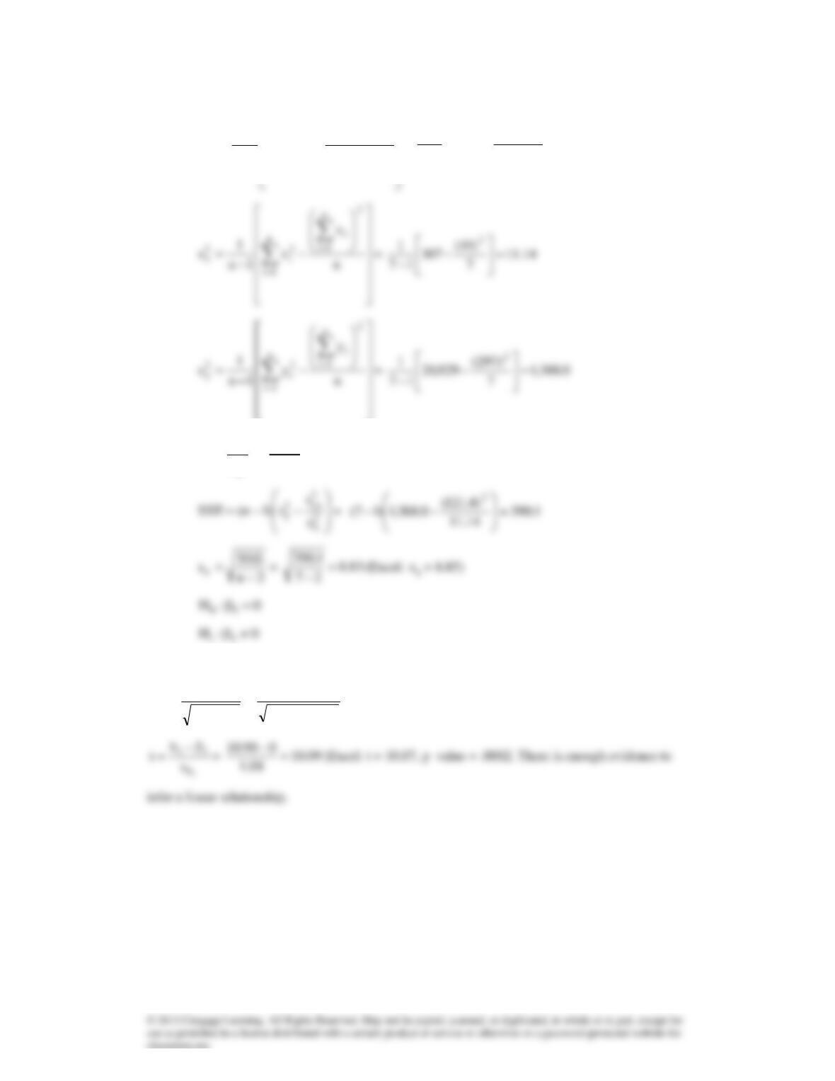
−
−
=
==
=n
yx
yx
1n
1
s
n
1i
i
n
1i
i
n
1i
iixy
=
4.121
7
297)(41(
468,2
17
1=
−
−
2
x
xy
1s
s
b=
=
90.10
14.11
4.121 =
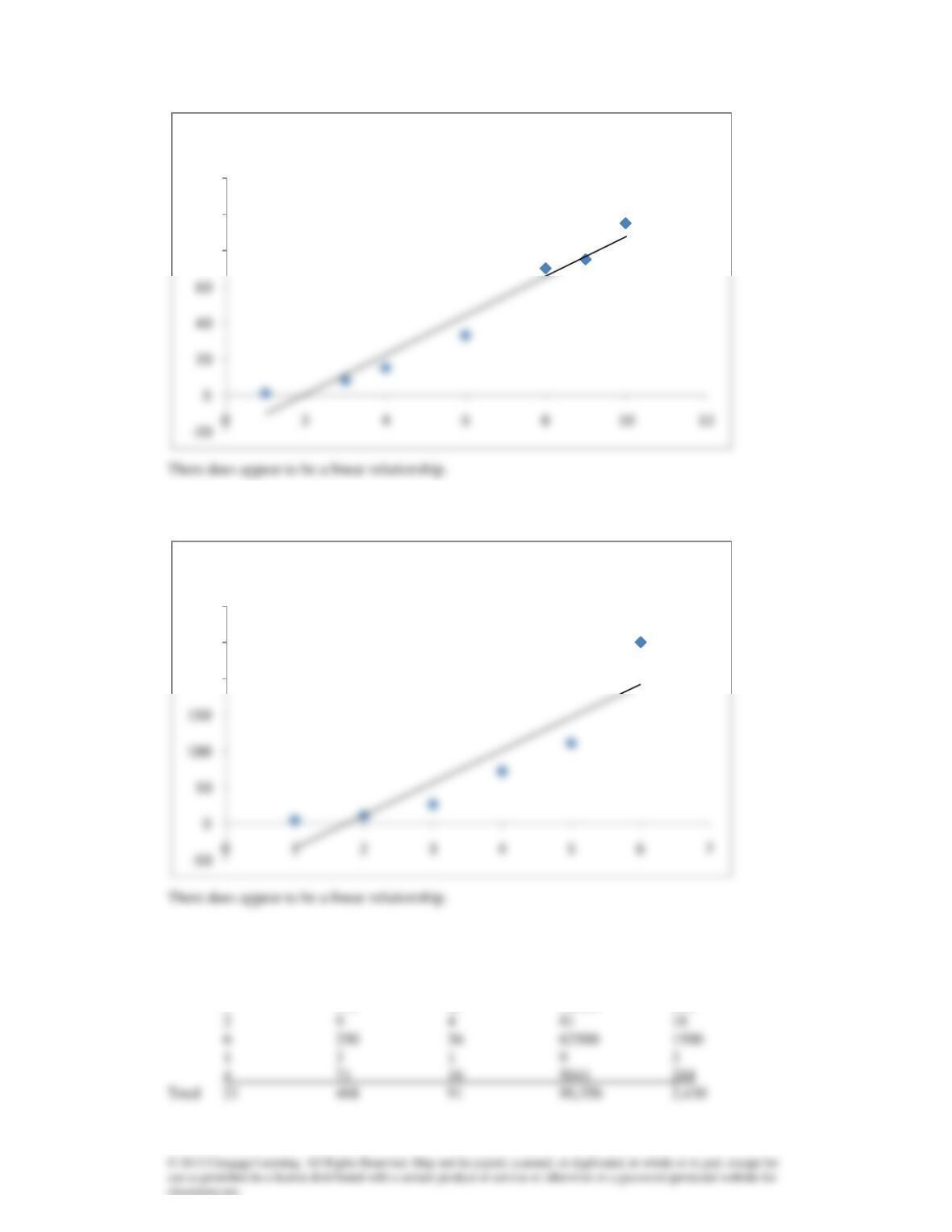
Rejection region:
571.2ttt 5,0 25.2n,2/ == −
or
571.2ttt 5,025.2n,2/ −=−=− −
2
x
b
s)1n(
s
s1−
=
=
08.1
)14.11)(17(
83.8 =
−
16.23a
b
i
x
i
y
2
i
x
2
i
y
iiyx
3 25 9 625 75
5 110 25 12100 550
80
100
120
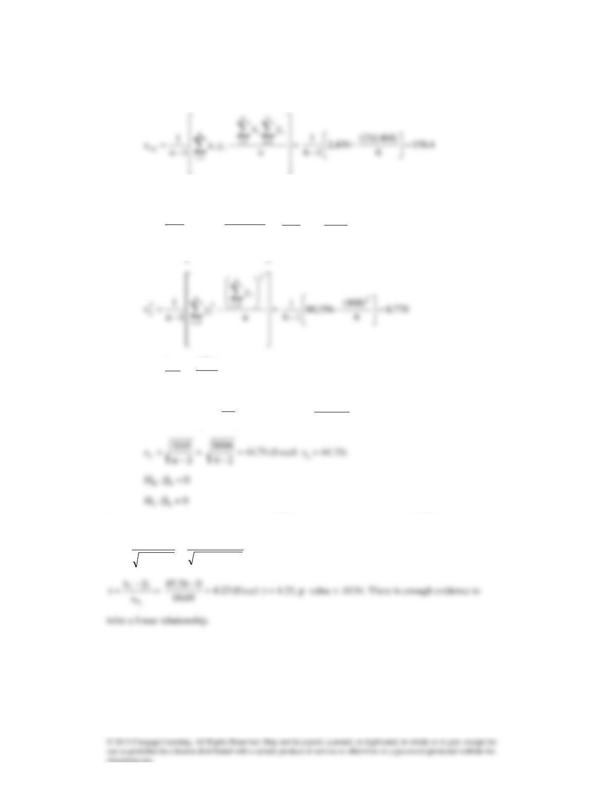
Scatter Diagram
200
250
300
Scatter Diagram
=
n
1i
i
x
= 21
=
n
1i
i
y
= 468
=
n
1i
2
i
x
= 91
=
n
1i
2
i
y
= 80,356
=
n
1i
ii yx
= 2,430
−
−
=
=
=n
x
x
1n
1
s
2
n
1i
i
n
1i
2
i
2
x
=
50.3
6
)21(
91
16
12
=
−
−
2
x
xy
1s
s
b=
=
26.45
5.3
4.158 =
−−= 2
x
2
xy
2
ys
s
s)1n(SSE
=
006,8
50.3
)4.158(
770,8)16(
2
=
−−
Rejection region:
776.2ttt 4,025.2n,2/ == −
or
776.2ttt 4,025.2n,2/ −=−=− −
2
x
b
s)1n(
s
s1−
=
=
69.10
)50.3)(16(
74.44 =
−
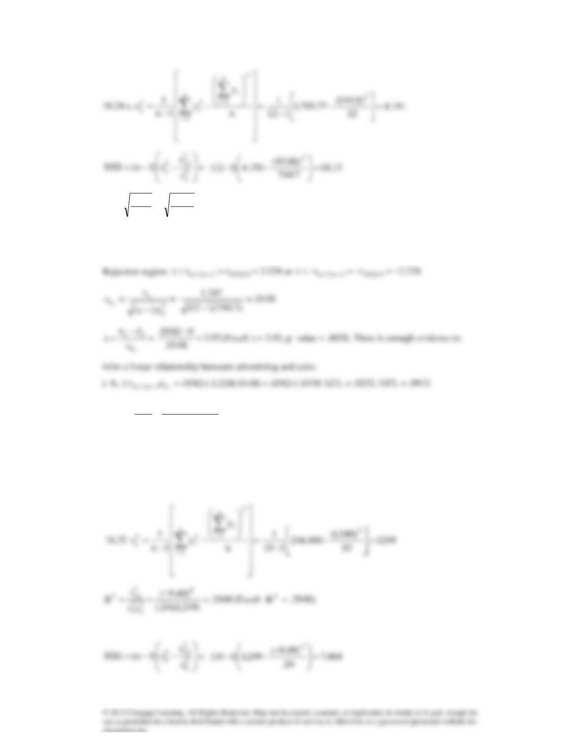
2n
SSE
s−
=
=
347.1
212
13.18 =
−
(Excel:
s
= 1.347)
b
0:H 10 =
0:H 11
d
2
y
2
x
2
xy
2
ss
s
R=
=
6067.
)191.4)(7.749(
)66.43(2
=
(Excel:
2
R
= .6066). 60.67% of the variation in sales is
explained by the variation in advertising.
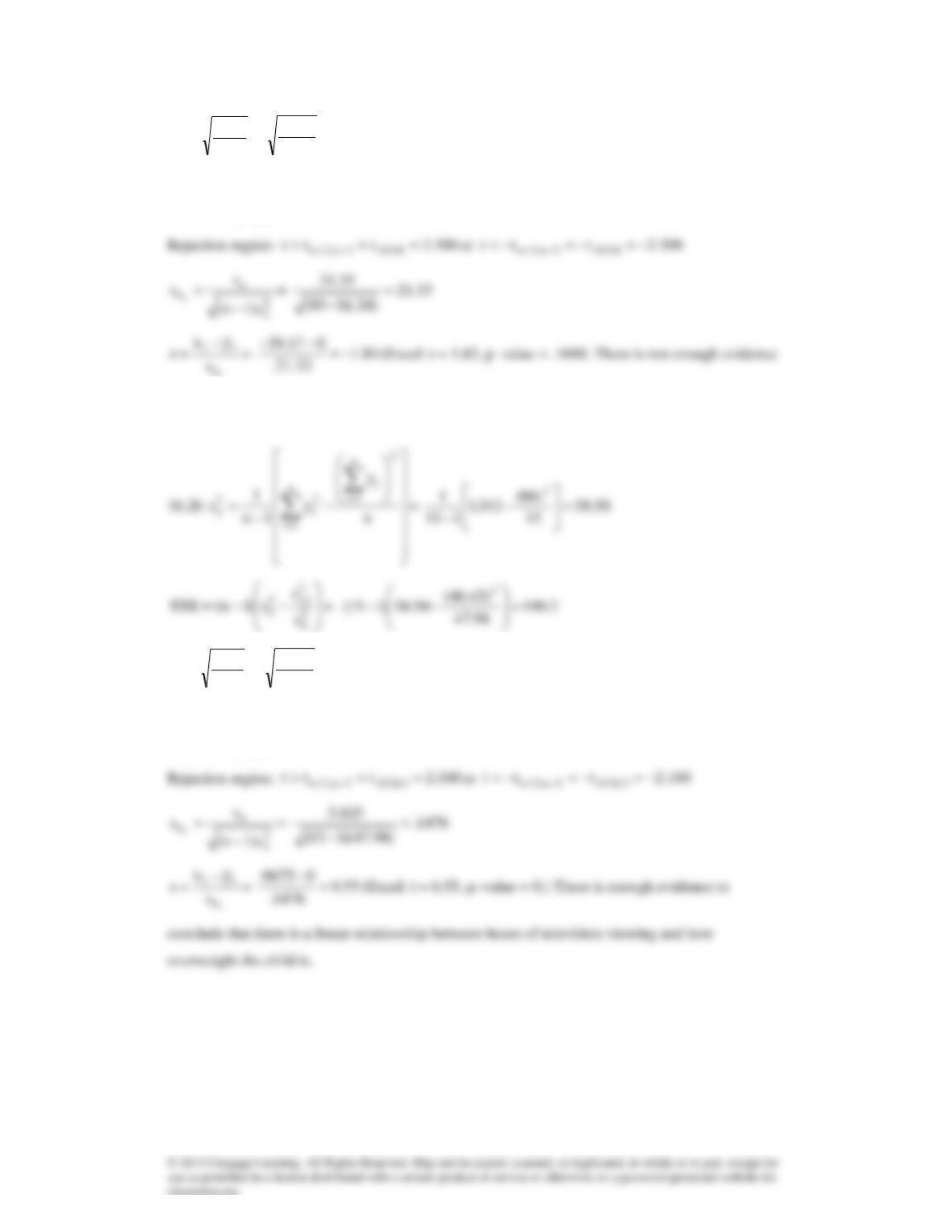
e There is evidence of a linear relationship. For each additional dollar of advertising sales increase,
on average by .0582.
2
y
2
x
2
xy
2
ss
s
R=
2
R
2n
SSE
s−
=
=
35.31
210
864,7 =
−
(Excel:
s
= 31.48)
0:H 10 =
0:H 11
1
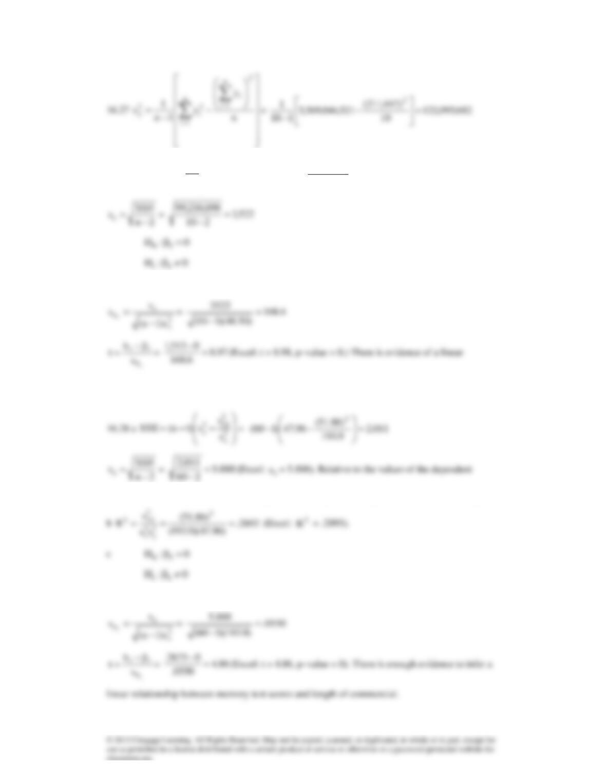
to infer a linear relationship between interest rates and housing starts.
2n
SSE
s−
=
=
825.3
215
2.190 =
−
0:H 10 =
0:H 11
1
−−= 2
x
2
xy
2
ys
s
s)1n(SSE
=
698,216,99
50.48
)396,73(
682,095,122)110(
2
=
−−
Rejection region:
306.2ttt 8,025.2n,2/ == −
or
306.2ttt 8,025.2n,2/ −=−=− −
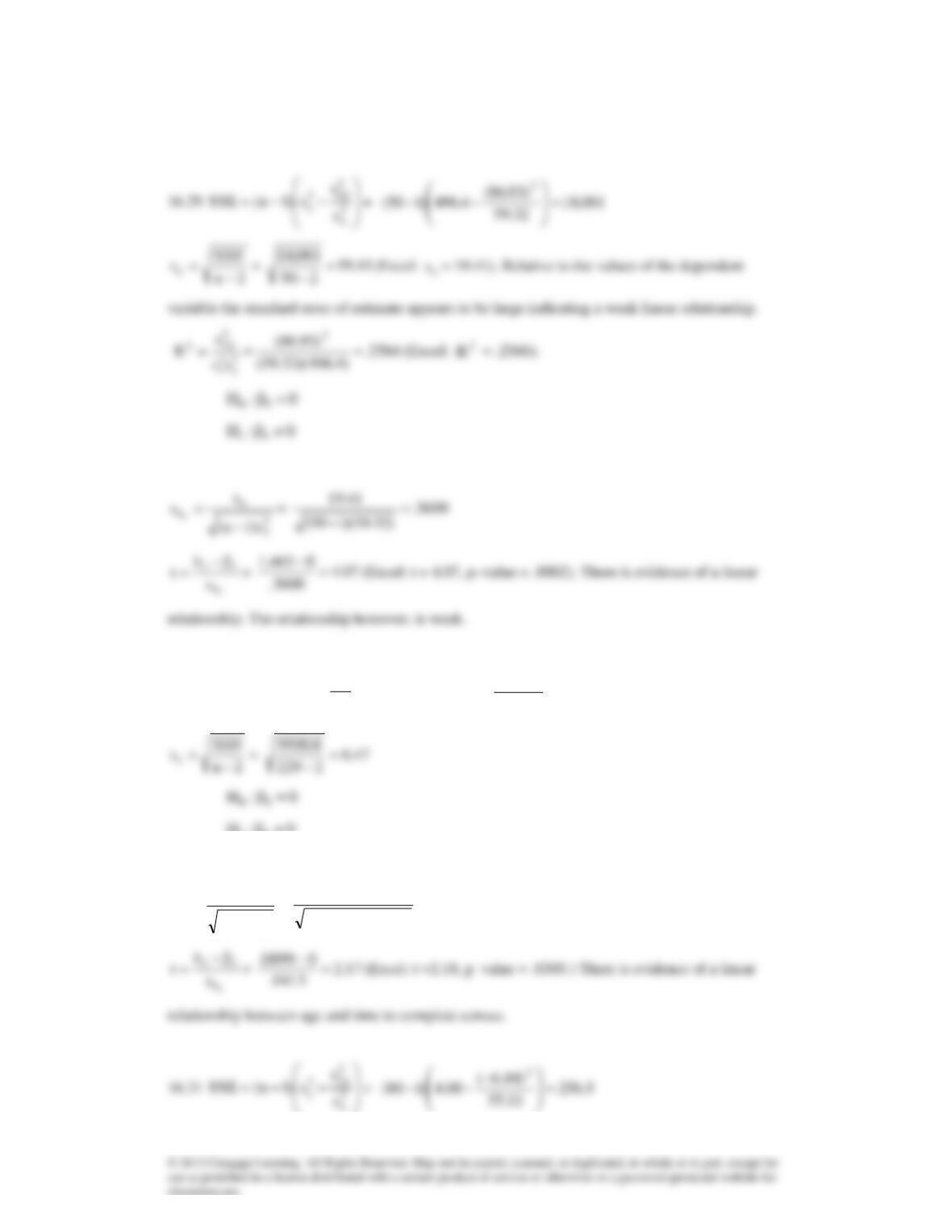
relationship between temperature and the number of beers sold.
variable the standard error of estimate appears to be large indicating a weak linear relationship.
Rejection region:
000.2ttt 58,025.2n,2/ = −
or
000.2ttt 58,025.2n,2/ −=−=− −
d
0919.2675.)0550(.671.12675.stb 1
b2n,2/1 == −
LCL = .1756, UCL = .3594
0:H 11
Rejection region:
009.2ttt 48,025.2n,2/ = −
or
009.2ttt 48,025.2n,2/ −=−=− −
16.30
−−= 2
x
2
xy
2
ys
s
s)1n(SSE
=
8.9500
51.107
)67.9(
54.42)1229(
2
=
−−
0:H 11
Rejection region:
96.1ttt 22 7,025.2n,2/ = −
or
96.1ttt 227,025.2n,2/ −=−=− −
2
x
b
s)1n(
s
s1−
=
=
0413.
)51.107)(1229(
47.6 =
−
2n
SSE
16.32
−−= 2
x
2
xy
2
ys
s
s)1n(SSE
=
3657
3.108
)55.20(
80.19)1231(
2
=
−−
2n
SSE
s−
=
=
996.3
2231
3657 =
−
2
s)1n(
s1−
16.33
−−= 2
x
2
xy
2
ys
s
s)1n(SSE
=
234,10
270.4
)83.22(
9.243)185(
2
=
−−
2n
SSE
Rejection region:
990.1ttt 83,02 5.2n,2/ = −
or
990.1ttt 83,025.2n,2/ −−=− −
2
x
b
s)1n(
s
s1−
=
=
5861.
)270.4)(185(
10.11 =
−
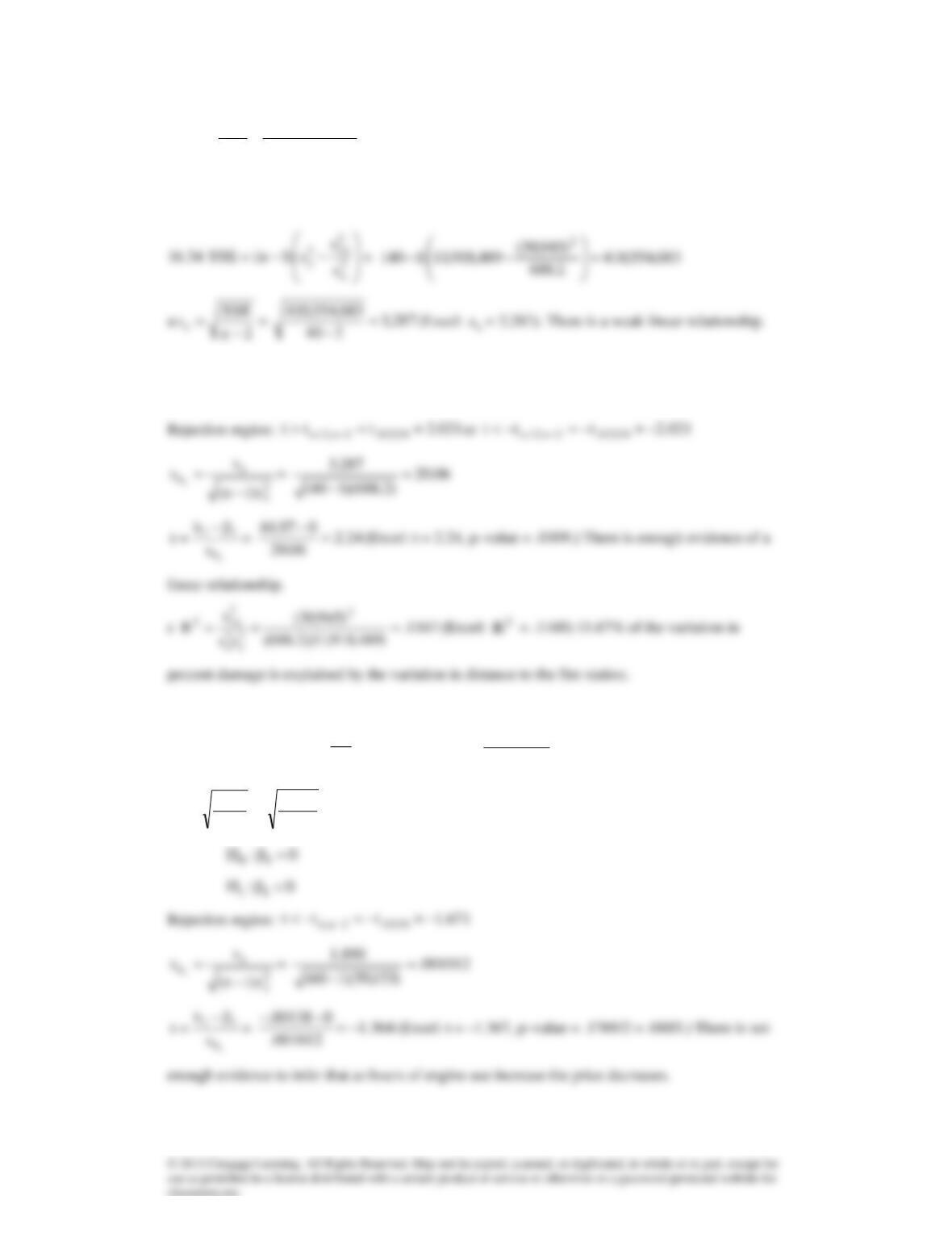
c
2
y
2
x
2
xy
2
ss
s
R=
=
5005.
)9.243)(270.4(
)83.22(2
=
(Excel:
2
R
= .5004). There is a moderately strong linear
relationship between distance and fire damage.
2n
SSE
s
b
0:H 10 =
0:H 11
2
y
2
x
ss
2
R
16.35
−−= 2
x
2
xy
2
ys
s
s)1n(SSE
=
1.207
153,59
)78.81(
623.3)160(
2
=
−
−−
2n
SSE
s−
=
=
890.1
260
1.207 =
−
(Excel:
s
=1.889 ).
0:H 10 =
0:H 11
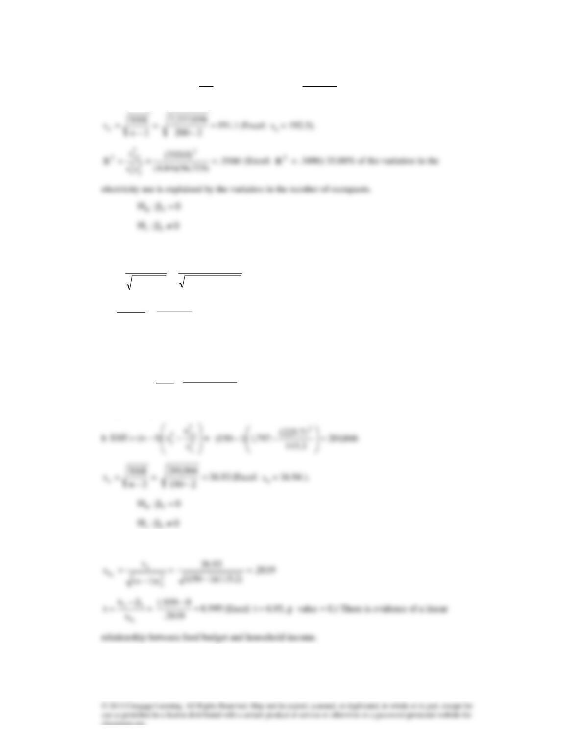
16.36
−−= 2
x
2
xy
2
ys
s
s)1n(SSE
=
056,337,7
84.4
)0.310(
725,56)1200(
2
=
−−
2
y
2
xy
2
ss
s
Rejection region:
972.1ttt 198,025.2n,2/ = −
or
972.1ttt 198,025.2n,2/ −−=− −
2
x
b
s)1n(
s
s1−
=
=
16.6
)84.4)(1200(
1.191 =
−
1
b
11
s
b
t−
=
=
39.10
16.6
005.64 =
−
(Excel: t =10.32, p–value = 0.) There is enough evidence of a
linear relationship.
16.37 a
2
y
2
x
2
xy
2
ss
s
R=
=
2461.
)797,1)(2.115(
)7.225( 2
=
(Excel:
2
R
= .2459) 24.61% of the variation in food
budgets is explained by the variation in household income.
Rejection region:
977.1ttt 148,025.2n,2/ = −
or
977.1ttt 148,025.2n,2/ −−=− −
s)1n(
s
s1−
=
1
b
11
s
b
t−
=
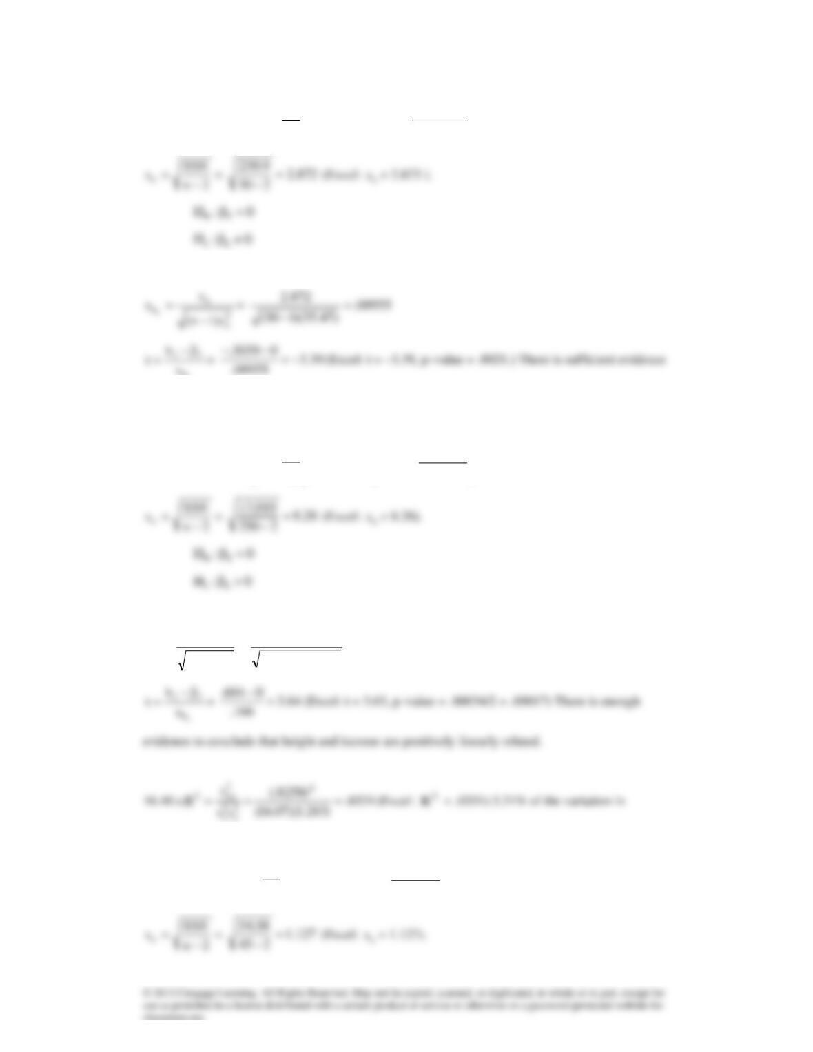
16.38
−−= 2
x
2
xy
2
ys
s
s)1n(SSE
=
9.230
47.35
)78.10(
24.11)130(
2
=
−
−−
Rejection region:
048.2ttt 28,025.2n,2/ == −
or
048.2ttt 28,025.2n,2/ −=−=− −
1
b
to conclude that office rents and vacancy rates are linearly related.
16.39
−−= 2
x
2
xy
2
ys
s
s)1n(SSE
=
010,17
966.9
)020.6(
95.71)1250(
2
=
−−
Rejection region:
645.1ttt 24 8,05.2n, = −
2
x
b
s)1n(
s
s1−
=
=
166.
966.9)(1250(
28.8 =
−
percentage of defectives is explained by the variation in aptitude test scores.
b.
−−= 2
x
2
xy
2
ys
s
s)1n(SSE
=
58.54
07.16
)8258(.
283.1)145(
2
=
−−
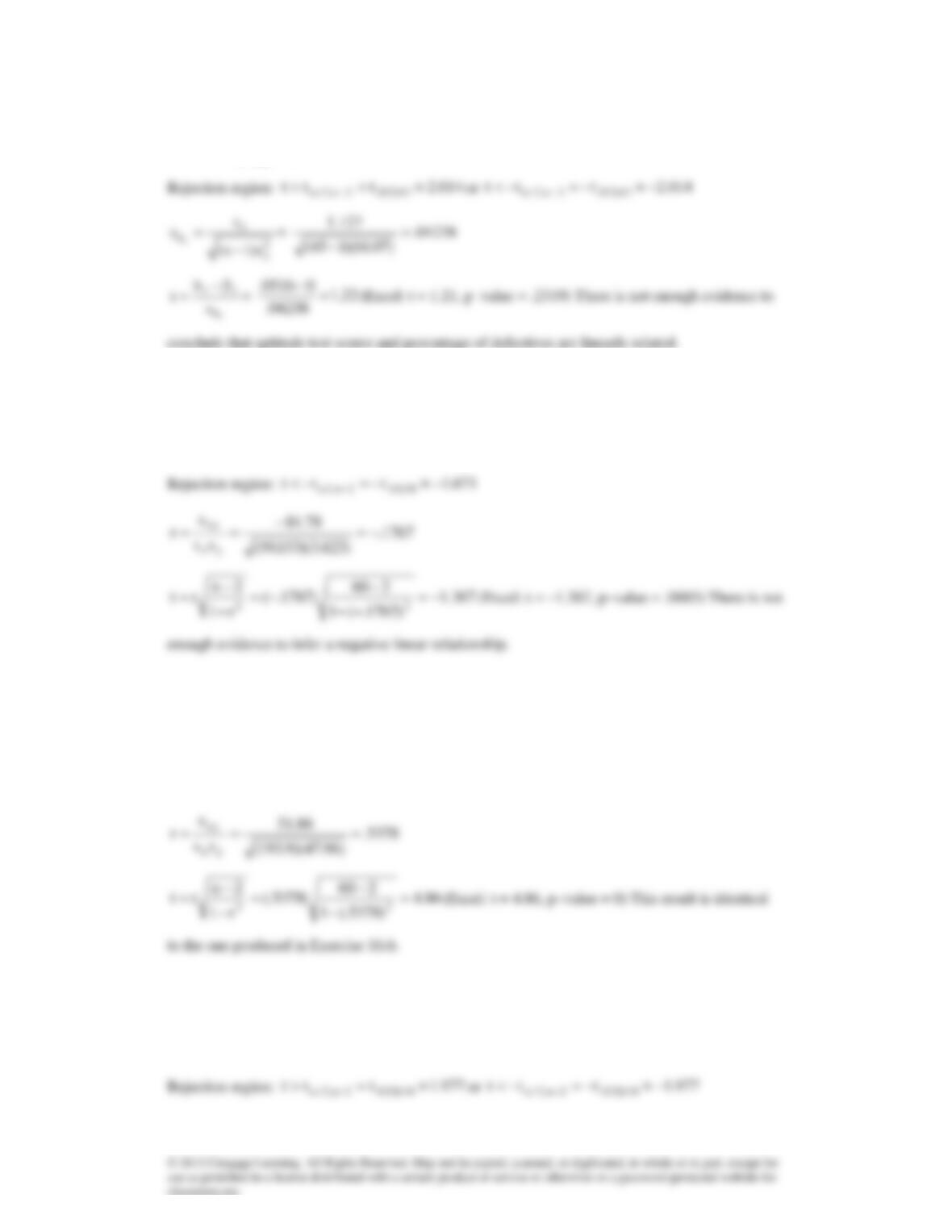
0:H 10 =
0:H 11
014.2ttt 43,025.2n,2/ −−=− −
16.41
0:H0=
0:H1
16.42
0:H0=
0:H1
Rejection region:
000.2ttt 58,025.2n,2/ = −
or
000.2ttt 58,025.2n,2/ −=−=− −
16.43
0:H0=
0:H1