│ CASE STUDY 513
CHAPTER 1
CASE STUDY:
RATING TELEVISION SHOWS IN THE UNITED STATES
1. Yes. A rating of 8.4 is equivalent to 9,618,000 households which is twice the number of
households at a rating of 4.2.
5. Day, Time
Data can be chronologically ordered.
Hours or minutes
6. Rating, Share, and Audience
CHAPTER 2
CASE STUDY:
EARNINGS OF ATHLETES
1. The NFL because it has a lot more players than the other organizations.
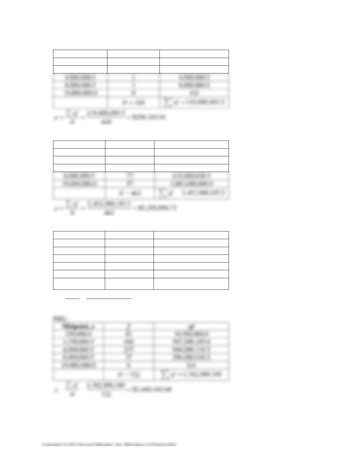
2. MLB:
Midpoint, x f xf
250,000.0 353 88,250,000.0
514 CASE STUDY │
MLS:
Midpoint, x f xf
250,000.0 403 100,750,000.0
1,250,000.5 5 6,250,002.5
NBA:
Midpoint, x f xf
250,000.0 35 8,750,000.0
1,250,000.5 157 196,250,078.5
4,000,000.5 137 548,000,068.5
NFL:
Midpoint, x f xf
250,000.0 554 138,500,000.0
1,250,000.5 746 932,500,373.0
4,000,000.5 438 1,752,000,219.0
8,000,000.5 85 680,000,042.5
19,000,000.0 38 722,000,000.0
1861N= 4,225,000,592.5xf =
∑
4, 225, 000,592.5 $2,270,285.11
1861
xf
N
µ∑
== ≈
│ CASE STUDY 515
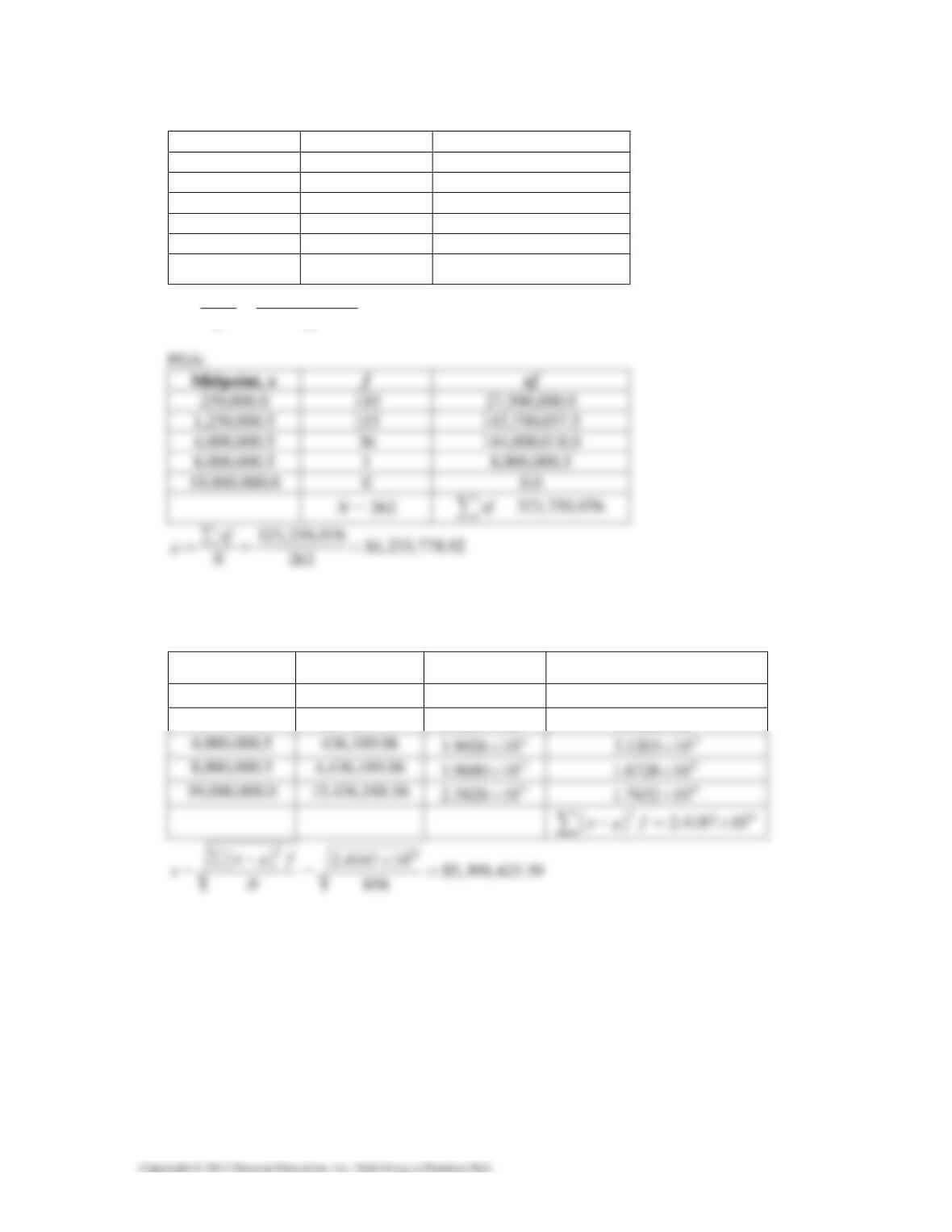
NASCAR:
Midpoint, x f xf
250,000.0 23 5,750,000.0
1,250,000.5 16 20,000,008.0
4,000,000.5 31 124,000,015.5
8,000,000.5 6 48,000,003.0
19,000,000.0 0 0.0
76N= 197,750,026.5xf =
∑
197,750,026.5 $2,601,974.03
76
xf
N
µ∑
== ≈
3. The NBA had the greatest earnings per player ($5,295,896.73).
4. MLB: $3,563,811.44µ≈
Midpoint, x
x
µ−
(
)
2
xµ−
(
)
2
x
fµ−
250,000.0 –3,313,811.44 13
1.0981 10× 15
3.8764 10×
1,250,000.5 –2,313,810.94 12
5.3537 10× 14
9.7438 10×
516 CASE STUDY │
MLS: $290,243.91µ≈
Midpoint, x
x
µ−
(
)
2
xµ−
(
)
2
x
fµ−
250,000.0 –40,243.91 9
1.6196 10× 11
6.5269 10×
1,250,000.5 959,756.59 11
9.2113 10× 12
4.6057 10×
NBA: $5,295,896.73µ≈
Midpoint, x
x
µ−
(
)
2
xµ−
(
)
2
x
fµ−
250,000.0 –5,045,896.73 13
2.5461 10× 14
8.9114 10×
1,250,000.5 –4,045,896.23 13
1.6369 10× 15
2.5700 10×
NFL: $2,270,285.11µ≈
Midpoint, x
x
µ−
(
)
2
xµ−
(
)
2
x
fµ−
250,000.0 –2,020,285.11 12
4.0816 10× 15
2.2612 10×
1,250,000.5 –1,020,284.61 12
1.0410 10× 14
7.7657 10×
4,000,000.5 1,729,715.39 12
2.9919 10× 15
1.3105 10×
8,000,000.5 5,729,715.39 13
3.2830 10× 15
2.7905 10×
│ CASE STUDY 517
NHL: $2,440,443.68µ≈
Midpoint, x
x
µ−
(
)
2
xµ−
(
)
2
x
fµ−
250,000.0 –2,190,443.68 12
4.7980 10× 14
2.0152 10×
1,250,000.5 –1,190,443.18 12
1.4172 10× 14
5.7536 10×
NASCAR: $2,601,974.03µ≈
Midpoint, x
x
µ−
(
)
2
xµ−
(
)
2
x
fµ−
250,000.0 –2,351,974.03 12
5.5318 10× 14
1.2723 10×
1,250,000.5 –1,351,973.53 12
1.8278 10× 13
2.9245 10×
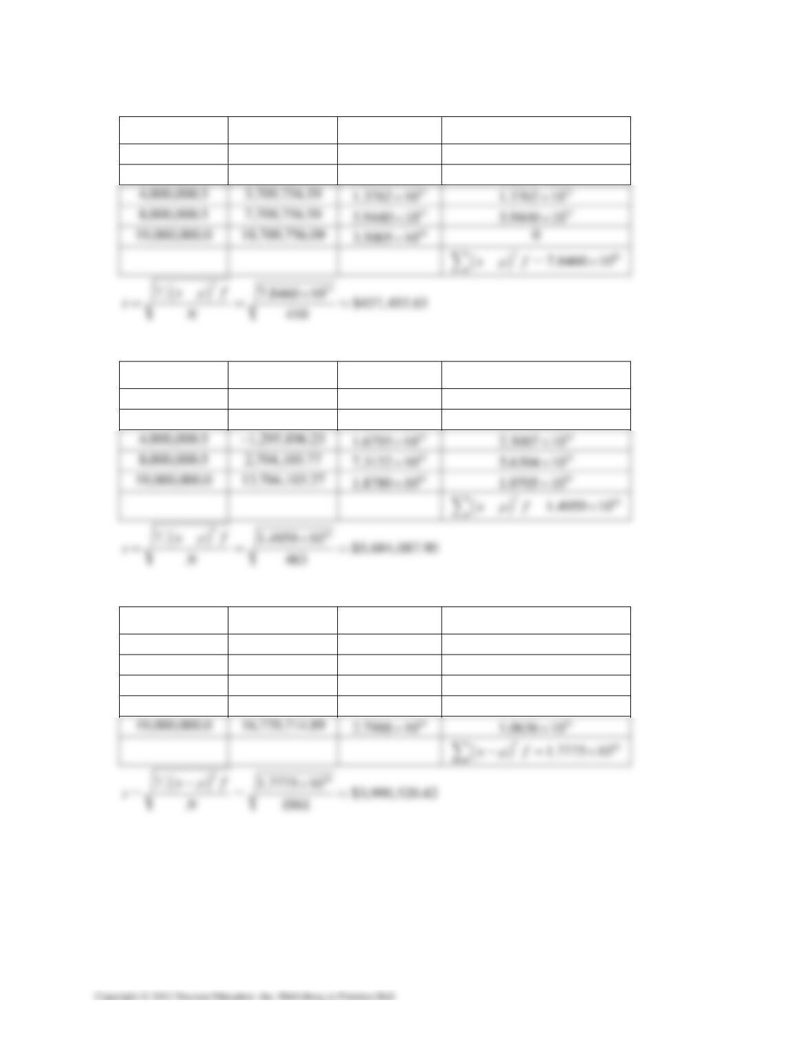
PGA: $1,233,778.92µ≈
Midpoint, x
x
µ−
(
)
2
xµ−
(
)
2
x
fµ−
250,000.0 –983,778.92 11
9.6782 10× 14
1.0646 10×
1,250,000.5 16,221.58 8
2.6314 10× 10
3.0261 10×
4,000,000.5 2,766,221.58 12
7.6520 10× 14
2.7547 10×
8,000,000.5 6,766,221.58 13
4.5782 10× 13
4.5782 10×
19,000,000.0 17,766,221.08 14
3.1564 10× 0
()
214
4.2774 10xfµ−= ×
∑
518 CASE STUDY │
CHAPTER 3
CASE STUDY:
UNITED STATES CONGRESS
1. P(female representative) 76 0.176
433
==
P(female senator) 17 0.17
100
==
4. (a) P(male senator) 83 0.83
100
==
(b) P(senator is not a Democrat) 43 0.43
100
==
(c) P(female or Republican)
()( )( )
female Republican female and Republican
17 41 4 0.54
100 100 100
PP P=+ −
=+−=
(d) P(male or Democrat)
()( )( )
male Democrat male and Democrat
83 57 44 0.96
100 100 100
PP P=+ −
=+−=
(e) Mutually exclusive. In the 111th Congress, a senator cannot be both female and Independent
because there are no female Independent senators.
│ CASE STUDY 519
CHAPTER 4
CASE STUDY:
BINOMIAL DISTRIBUTION OF AIRPLANE ACCIDENTS
1. P(crash in 2006) = 20.00000018
11,000,000 ≈
3. n = 11,000,000, p = 0.0000008
(a) P(x = 4) ≈ 0.0376641
(b) P(x= 10) ≈ 0.1156838
(c) P(1 ≤ x ≤ 5) ≈ 0.1282358
x P(x)
0 0.0001507
1 0.0013264
2 0.0058364
3 0.0171200
4. No, because each flight is not an independent trial. There are no flights that use the same plane.
520 CASE STUDY │
CHAPTER 5
CASE STUDY:
BIRTH WEIGHTS IN AMERICA
1. (a) 42 weeks and over
()
7.57µ=
(b) 32 to 33 weeks
()
5.14µ=
(c) 41 weeks
()
7.75µ=
3. (a) Top 10% ⇒ 90th percentile ⇒ z = 1.28
1.90 (1.28)(1.22) 3.46xzµσ=+ = + =
Birth weights must be at least 3.46 pounds to be in the top 10%.
(b) Top 10% ⇒ 90th percentile ⇒ z = 1.28
6.19 (1.28)(1.29) 7.84xzµσ=+ = + =
Birth weights must be at least 8.99 pounds to be in the top 10%.
4. (a) (6 9) (3.36 5.82) 1 0.9996 0.0004Px P z<< = << ≈− =
(b)
(6 9) (1.01 2.61) 0.9955 0.8438 0.1517Px P z<< = << = − =
(c)
(6 9) ( 0.15 2.18) 0.9854 0.4404 0.5450Px P z<< = − << = − =
(d)
(6 9) ( 1.19 1.58) 0.9429 0.1170 0.8259Px P z<< = − << = − =
│ CASE STUDY 521
CHAPTER 6
CASE STUDY:
MARATHON TRAINING
2. (a) 8.36
σ
≈
(b) 7.90
σ
≈
4. (a) With 95% confidence, you can say the mean male training time is between 164.9 and 170.9
minutes.
(b) With 95% confidence, you can say the mean female training time is between 186.2 and 191.8
minutes.
5. 178.45x=
13.35
σ
≈
13.35
178.45 1.96 178.45 3.38 (175.07, 181.83)
60
c
xz n
σ
±≈ ± ≈ ±≈
CHAPTER 7
CASE STUDY:
HUMAN BODY TEMPERATURE: WHAT’S NORMAL?
1. (a) (see part d)
(b)
01.96z=± (see part d)
(c) Rejection regions: 1.96z<− and 1.96z> (see part d)
522 CASE STUDY │
(d) 98.25,x≈ 0.73s≈
98.25 98.6 0.35 5.469
0.73 0.0640
130
x
zs
n
µ−−−
== = ≈−
2. No, 0
0.01 2.575zα=→=± →Reject 0
H
3. 0: 98.6 and : 98.6
mam
HHµµ=≠
0
0.01 2.575zα=→=±
98.105,x≈ 0.699s≈
98.105 98.6 0.495 5.709
0.699 0.0867
65
x
zs
n
µ−−−
== = ≈−
Reject
0
H. There is sufficient evidence to reject the claim.
│ CASE STUDY 523
CHAPTER 8
CASE STUDY:
READABILITY OF PATIENT EDUCATION MATERIALS
1. 01 2 1 2
:; : (claim)
A
HH
µ
µµµ
=≠
01.96;z=± Rejection regions: 1.96, 1.96zz<− >
µ
2. 01 3 1 3
:; : (claim)
A
HH
µ
µµµ
=≠
01.96;z=± Rejection regions: 1.96, 1.96zz<− >
µ
3. 02 3 2 3
:; : (claim)
A
HH
µ
µµµ
=≠
01.96;z=± Rejection regions: 1.96, 1.96zz<− >
µ
524 CASE STUDY │
5.
22 22
12 12
12 1 2 12
12 12
() ()
cc
ss ss
xx z xx z
nn nn
µµ
−− +<−<−+ +
6. (a) 01 4 1 4
:; : (claim)
A
HH
µ
µµµ
=≠
02.575;z=± Rejection regions: 2.575, 2.575zz<− >
µ
(b)
02 4 2 4
:; : (claim)
A
HH
µ
µµµ
=≠
02.575;z=± Rejection regions: 2.575, 2.575zz<− >
µ
CHAPTER 9
CASE STUDY:
CORRELATION OF BODY MEASUREMENTS
1. Answers will vary.
│ CASE STUDY 525
2.
r
a 0.698
b 0.746
c 0.351
3. d, g, and j have strong correlations (r > 0.8).
(d)
1.129 8.817yx=−
(g)
1.717 23.144yx=+
(j)
1.279 10.451yx=+
5. (weight, chest) r = 0.888
(weight, hip) r = 0.930
(neck, wrist) r = 0.849
(chest, hip) r = 0.953
(chest, thigh) r = 0.936
526 CASE STUDY │
CHAPTER 10
CASE STUDY:
FAST FOOD SURVEY
Gender Expected Frequencies:
Response Female Male Total
Somewhat Agree 272.214 127.786 400
1. Females exceeded the expected number of “somewhat agree” responses, males did not.
2. Females exceeded the expected number of neither agree nr disagree” responses, males did not.
3. 0:H Response is independent of gender.
:
a
H Response is dependent on gender.
0.01,
α
= d.f. = (r − 1)((c − 1) = 3 ⇒ 2
07.815
χ
=
O E O
−
E OE
2
()− OE
E
2
()−
286 272.214 13.786 190.053796 0.6982
114 127.786 −13.786 190.053796 1.4873
76 91.192
215,167
χ
≈
Reject
0.H There is enough evidence at the 1% level of significance to support the claim that
response and gender are dependent.
│ CASE STUDY 527
Response Distribution O E O
−
E OE
2
()− OE
E
2
()−
Somewhat Agree 59% 286 270.22 15.78 249.0084 0.9215
25.745
χ
≈
Fail to reject 0.H There is enough evidence at the 5% level of significance to that the distribution
of female responses matches the national distribution.
Response Distribution O E O
−
E OE
2
()− OE
E
2
()−
Somewhat Agree 59% 114 126.85 15.78 249.00854 1.3017
Neither agree or
disagree 20% 58 43.00
−15.60 243.3600 5.2326
29.444
χ
≈
Reject
0.H There is enough evidence at the 5% level of significance to conclude that the
distribution of male responses differs from the national distribution.
528 CASE STUDY │
CHAPTER 11
CASE STUDY:
COLLEGE RANKS
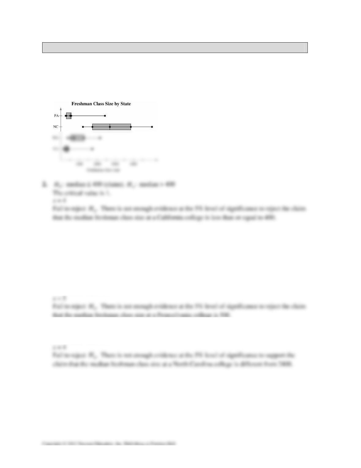
1. Using a technology, tool it appears the median freshman class size of North Carolina is different
from the other states.
3. 0:H median ≥ 750 (claim); :
a
H median < 750
The critical value is 1.
x = 5
Fail to reject 0.H There is not enough evidence at the 5% level of significance to reject the claim
that the median freshman class size at a Massachusetts college is greater than or equal to 750.
4. 0:H median = 500 (claim); :
a
H median ≠ 500
The critical value is 1.
5. 0:H median = 2400 (claim); :
a
H median ≠ 2400
The critical value is 1.
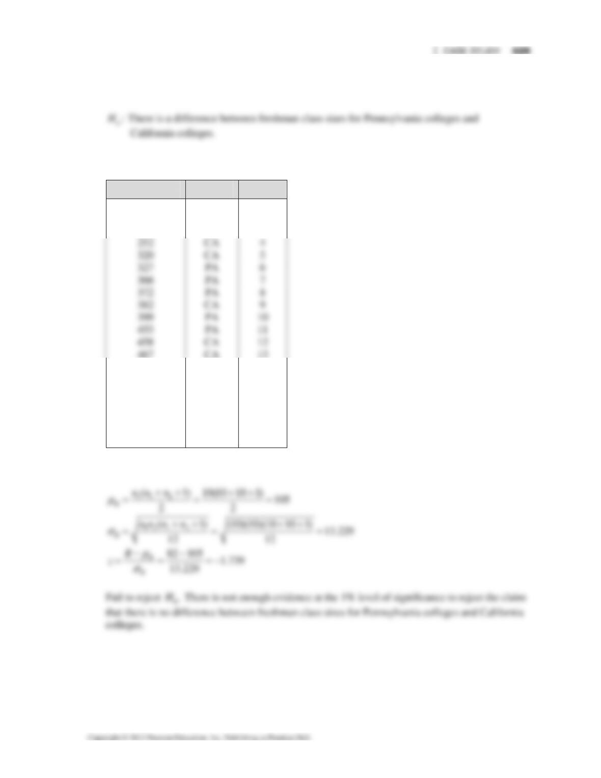
6. 0:H There is no difference between freshman class sizes for Pennsylvania colleges and
California colleges. (claim)
02.575z=±
R = sum ranks of California = 82
Ordered Data Sample Rank
202 CA 1.5
202 CA 1.5
236 CA 3
574 CA 14
588 PA 15
601 PA 16
613 PA 17
957 PA 18
1703 CA 19
2400 PA 20
530 CASE STUDY │
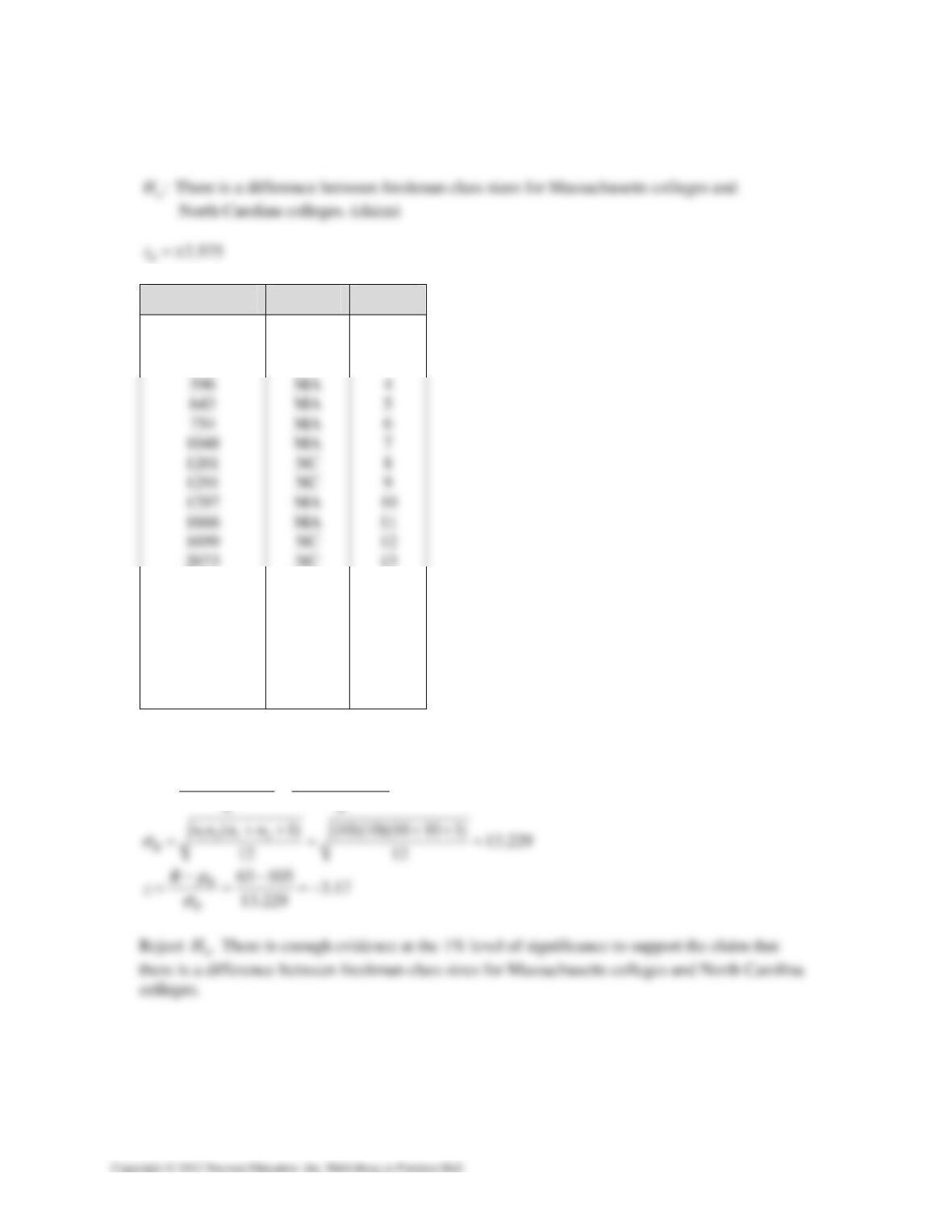
7. 0:H There is no difference between freshman class sizes for Massachusetts colleges and
North Carolina colleges.
Ordered Data Sample Rank
439 MA 1
518 MA 2
540 MA 3
2167 MA 14
2492 NC 15
2781 NC 16
3090 NC 17
3865 NC 18
4538 NC 19
4804 NC 20
R = sum ranks of Massachusetts = 63
11 2
(1)
10(10 10 1) 105
22
R
nn n
µ
++ ++
== =