1
CHAPTER 16
Problem 16.1
Solve the problem in Example 16.1 by the central
difference method, implemented by a computer program in
a language of your choice using ∆t = 0.1 sec.
First we set up modal equations. These are given by
Eq. (16.2.3) with M, C,
K
, and
tP available from
Example 16.1:
The first two natural frequencies and modes are given by
1.0 Initial calculations.
8.102
1.7 Substituting M, C,
K
, and tΔin step 1.7 in
Table 16.2.1 gives
2.0 Calculations for each time step i.
1.067 ()
Pu
2.3 Solve:
1
2
1
i
i
iq
The resulting modal displacements i
q are given in Table

2
Table P16.1: Numerical solution of modal equations by the central difference method
i
t 1
q 2
q 1
u 2
u 3
u 4
u 5
u
0.
1
0
0.0000
0.0000
0.0000
0.0000
0.0000
0.0000
0.0000
0.30
–
3.8393
–
3.8393
–
1.5983
–
2.8740
–
3.6642
–
4.0195
–
4.1211
–
–
–
–
–
–
–
0.50
–
9.1914
–
9.1914
–
3.0850
–
5.9097
–
8.2420
–
9.8991
–
10.7581
–
–
–
–
–
–
–
0.70
–
3.8833
–
3.8833
–
0.9976
–
2.0963
–
3.2634
–
4.2963
–
4.9133
0.90 11.2485 11.2485 3.8374 7.3135 10.1309 12.0915 13.0913
1.10 16.2401 16.2401 5.3357 10.2909 14.4802 17.5335 19.1470
1.30 2.9823 2.9823 1.0480 1.9791 2.7079 3.1944 3.4341
1.50
–
12.1266
–
12.1266
–
4.0557
–
7.7780
–
10.8636
–
13.0656
–
14.2110
–
–
–
–
–
–
–
1.70
–
12.4039
–
12.4039
–
4.1674
–
7.9806
–
11.1256
–
3.3574
–
14.5133
–
–
–
–
–
–
–
Problem 16.2
time step affect the accuracy of the solution?
Solution:
1.1 Since the system starts from rest, 0uu
00 ;
therefore, 0qq 00 .
1.4 05.0Δ t sec.
1.6 Substituting M, C, and tΔin step 1.6 of Table
16.2.1 gives
1.7 Substituting M, C,
K
, and tΔin step 1.7 of
Table 16.2.1 gives
2.0 Calculations for each time step i.
2.3 Solve:
The resulting modal displacements i
q are given in Table
2.5 11ii
uq
1
2
0.334 0.895
0.641 1.173
u
uq
These displacements are also presented in Table P16.2a.
3.0 Comments.

Table P16.2a: Numerical solution of modal equations by the central difference method
i
t 1
q 2
q 1
u 2
u 3
u 4
u 5
u
0.05 0.0000 0.0000 0.0000 0.0000 0.0000 0.0000 0.0000
0.15 –0.5960 –0.5960 –0.3362 –0.5615 –0.6318 –0.5912 –0.5338
0.25 –2.5340 –2.5340 –1.1711 –2.0492 –2.5016 –2.6096 –2.5801
0.35 –5.5264 –5.5264 –2.0965 –3.8696 –5.1284 –5.8619 –6.1777
0.45 –8.2551 –8.2551 –2.7774 –5.3165 –7.4072 –8.8882 –9.6542
0.55 –8.9614 –8.9614 –2.9037 –5.6254 –7.9612 –9.6902 –10.6143
0.65 –6.3610 –6.3610 –1.9848 –3.8931 –5.5965 –6.9067 –7.6260
0.75 –0.4529 –0.4529 0.0996 0.0383 –0.2262 –0.5816 –0.8329
0.85 7.1843 7.1843 2.6638 4.9499 6.6228 7.6433 8.1050
0.95 13.8108 13.8108 4.6924 8.9543 12.4249 14.8529 16.0964
1.05 16.5462 16.5462 5.4113 10.4522 14.7353 17.8732 19.5378
1.15 14.1986 14.1986 4.6915 9.0321 12.6790 15.3195 16.7081
1.25 7.7447 7.7447 2.6893 5.0973 7.0090 8.3074 8.9566
1.35 –0.6678 –0.6678 –0.2033 –0.4021 –0.5839 –0.7270 –0.8067
1.45 –8.4236 –8.4236 –2.9042 –5.5167 –7.6084 –9.0435 –9.7669
1.55 –13.2455 –13.2455 –4.4192 –8.4816 –11.8584 –14.2753 –15.5353
1.65 –13.8554 –13.8554 –4.5465 –8.7723 –12.3498 –14.9609 –16.3422
1.75 –10.3002 –10.3002 –3.4554 –6.6203 –9.2350 –11.0940 –12.0582
1.85 –3.8669 –3.8669 –1.3536 –2.5593 –3.5074 –4.1439 –4.4589
1.95 3.3697 3.3697 1.1521 2.1942 3.0367 3.6213 3.9187
5
Table P16.2b
i
t )1.0Δ(
5tu )05.0Δ(
5
tu
5
u
(Theoretical)
0.10 0.0000 –0.1322 –0.1804
0.30 –4.1211 –4.2516 –4.2998
0.50 –10.7581 –10.5746 –10.4925
0.70 –4.9133 –4.6370 –4.5850
0.90 13.0913 12.4524 12.2796
1.10 19.1470 18.8818 18.7924
1.30 3.4341 4.1378 4.3529
1.50 –14.2110 –13.1853 –12.8543
1.70 –14.5133 –14.7608 –14.8285
1.90 0.9855 –0.2129 –0.5740
Problem 16.3
Solve the problem in Example 16.1 by the constant average
acceleration method, implemented by a computer program
in a language of your choice using ∆t = 0.1 sec. Based on
K
1
559.0
The first two natural frequencies and modes are given by
Eq. (b) of Example 16.1. We now implement the procedure
of Table 16.2.2.
1.0 Initial calculations.
1.2 0p
0; therefore, 0P
0.
1.6 Substituting
K
and 1
a in step 1.6 of Table
16.2.2 gives
2.0 Calculations for each time step i.
For the parameters of this problem, computational
steps 2.1 through 2.5 are specialized and implemented for
each time step ias follows.
ˆ
5.442
P
qq
iiii q
2
1
1
2.5 11ii
uq
1
2
0.334 0.895
0.641 1.173
u
uq
These displacements are also presented in Table P16.3a.

7
Table P16.3a: Numerical Solution of modal equations by the average acceleration method
i
t 1
q 2
q 1
u 2
u 3
u 4
u 5
u
0.00 0.0000 0.0000 0.0000 0.0000 0.0000 0.0000 0.0000
0.20 –1.4463 –1.4463 –0.6780 –1.1822 –1.4347 –1.4858 –1.4610
0.40 –6.4838 –6.4838 –2.3938 –4.4537 –5.9697 –6.9020 –7.3272
0.60 –7.5677 –7.5677 –2.3093 –4.5636 –6.6210 –8.2364 –9.1354
0.80 2.4442 2.4442 0.9967 1.8024 2.3179 2.5667 2.6487
1.00 14.1522 14.1522 4.7892 9.1505 12.7183 15.2272 16.5173
1.20 11.6343 11.6343 3.8044 7.3487 10.3606 12.5676 13.7385
1.40 –2.5294 –2.5294 –0.7664 –1.5182 –2.2091 –2.7549 –3.0599
1.60 –12.7114 –12.7114 –4.3077 –8.2269 –11.4279 –13.6747 –14.8285
1.80 –8.8947 –8.8947 –2.9247 –5.6395 –7.9325 –9.6022 –10.4840
2.00 3.6390 3.6390 1.1943 2.3043 3.2438 3.9293 4.2919
Table P16.3b: Comparison of central difference and average
acceleration methods
i
t
)1.0Δ(
5tu
central diff.
)1.0Δ(
5tu
avg. accel.
5
u
(Theoretical)
0.00 0.0000 0.0000 0.0000
0.20 –1.0015 –1.4610 –1.4153
0.40 –8.2612 –7.3272 –8.0443
0.60 –9.8873 –9.1354 –9.5676
0.80 3.7100 2.6487 3.4995
1.00 19.1734 16.5173 18.3511
1.20 13.0638 13.7385 13.3779
1.40 –6.5775 –3.0599 –5.2533
1.60 –17.1212 –14.8285 –16.4102
1.80 –7.7123 –10.4840 –8.7981
2.00 9.0272 4.2919 7.2622
Problem 16.4
Repeat Problem 16.3 using ∆t = 0.05 sec. How does the
time step affect the accuracy of the solution?
Solution:
Equation (16.2.3) gives the modal equations with M,
C,
K
, and
tP defined in the solution of Problem 16.3.
1.0 Initial calculations.
1.2 0p
0; therefore, 0P
0.
1622
56.80
1.6 Substituting
K
and 1
a in step 1.6 of Table 16.2.2
gives
2.0 Calculations for each time step i.
For the parameters of this problem, computational
steps 2.1 through 2.5 are specialized and implemented for
each time step ias follows.
The resulting modal displacements i
q are given in Table
P16.4a.
21
4
0.334 0.895
1.078 0.334
i
u
u
3.0 Comments.
Table P16.4a: Numerical Solution of modal equations by the average acceleration method
i
t 1
q 2
q 1
u 2
u 3
u 4
u 5
u
0.05 –0.0385 –0.0385 –0.0221 –0.0368 –0.0411 –0.0380 –0.0340
0.15 –0.6719 –0.6719 –0.3523 –0.5980 –0.6932 –0.6763 –0.6338
0.25 –2.5612 –2.5612 –1.1590 –2.0388 –2.5108 –2.6468 –2.6375
0.35 –5.4343 –5.4343 –2.0927 –3.8460 –5.0652 –5.7525 –6.0371
0.45 –8.0448 –8.0448 –2.7364 –5.2199 –7.2397 –8.6507 –9.3725
0.55 –8.7238 –8.7238 –2.7859 –5.4229 –7.7210 –9.4485 –10.3820
0.65 –6.2419 –6.2419 –1.9147 –3.7771 –5.4682 –6.7897 –7.5229
0.75 –0.5787 –0.5787 0.0112 –0.1030 –0.3719 –0.6998 –0.9246
0.85 6.7862 6.7862 2.5044 4.6602 6.2474 7.2241 7.6700
0.95 13.2529 13.2529 4.5598 8.6672 11.9638 14.2317 15.3776
1.05 16.0961 16.0961 5.2938 10.2067 14.3556 17.3759 18.9706
1.15 14.1127 14.1127 4.5975 8.8915 12.5553 15.2513 16.6860
1.25 8.1037 8.1037 2.7687 5.2742 7.3015 8.7095 9.4263
1.35 0.0430 0.0430 0.1153 0.1597 0.1107 0.0087 –0.0711
1.45 –7.6001 –7.6001 –2.5881 –4.9352 –6.8416 –8.1714 –8.8508
1.55 –12.6102 –12.6102 –4.2990 –8.1949 –11.3552 –13.5564 –14.6798
1.65 –13.6612 –13.6612 –4.5190 –8.6968 –12.2027 –14.7378 –16.0696
1.75 –10.6567 –10.6567 –3.4772 –6.7213 –9.4847 –11.5144 –12.5931
1.85 –4.6928 –4.6928 –1.5986 –3.0480 –4.2248 –5.0453 –5.4644
1.95 2.3267 2.3267 0.7059 1.3977 2.0327 2.5338 2.8136
10
Table P16.4b
i
t )1.0Δ(
5tu )05.0Δ(
5tu
5
u
(Theoretical)
0.10 –0.2622 –0.2027 –0.1804
0.30 –4.0203 –4.2203 –4.2998
0.50 –9.6827 –10.2981 –10.4925
0.70 –4.7508 –4.6151 –4.5850
0.90 10.7273 11.8425 12.2796
1.10 17.7014 18.5650 18.7924
1.30 5.9726 4.7599 4.3529
1.50 –10.6512 –12.2445 –12.8543
1.70 –14.7035 –14.9049 –14.8285
1.90 –3.4436 –1.2961 –0.5740
11
Problem 16.5
Solve the problem in Example 16.1 by the linear accel-
eration method, implemented by a computer program in a
language of your choice using ∆t = 0.1 sec. Based on these
results and those from Problem 16.3, comment on the
relative accuracy of the linear acceleration and constant
average acceleration methods. Note that this problem was
solved as Example 16.1 and the results were presented in
Table E16.1.
Solution:
Solution to this problem is available as Example 16.1
in the textbook. Table P16.5 shows these results using
Table P16.5
i
t
)1.0Δ(
5tu
avg. accel.
)1.0Δ(
5tu
linear accel.
5
u
(Theoretical)
0.00 0.0000 0.0000 0.0000
0.20 –1.4610 –1.3357 –1.4153
0.40 –7.3272 –7.5893 –8.0443
0.60 –9.1354 –9.4087 –9.5676
0.80 2.6487 2.9758 3.4995
1.00 16.5173 17.3602 18.3511
1.20 13.7385 13.6304 13.3779
1.40 –3.0599 –4.2003 –5.2533
1.60 –14.8285 –15.5745 –16.4102
1.80 –10.4840 –9.8223 –8.7981
2.00 4.2919 5.8944 7.2622
Comments.
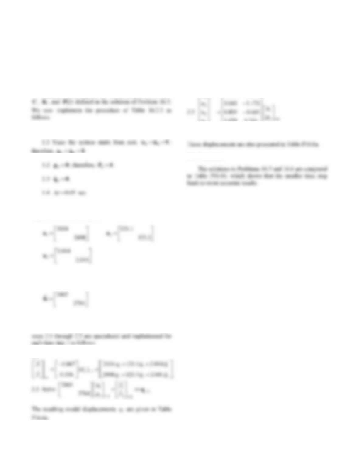
12
Problem 16.6
Repeat Problem 16.5 using ∆t = 0.05 sec. How does the
time step affect the accuracy of the solution?
Solution:
Equation (16.2.3) gives the modal equations with M,
1.0 Initial calculations.
1.5 Substituting M, C, tΔ, 2
1
, and 6
1
in
step 1.5 in Table 16.2.2 gives
1.6 Substituting
K
and 1
a in step 1.6 Table 16.2.2
gives
2.0 Calculations for each time step i.
For the parameters of this problem, computational
2.1
2.3 11111
22222
11
60 2 0.025
iiiii
qqqqq
qqqqq
2.4 11111
22222
11
2400 120 2
iiiii
qqqqq
qqqqq
1
5
4
078.1173.1
334.0078.1
895.0334.0
i
u
u
u
3.0 Comments.
K