16.116
Plot of Residuals vs Predicted
50
100
150
Histogram
20
Plot of Residuals vs Predicted
2
4
6
16.117
The error variable appears to be normal.
16.118
100
Histogram
10
15
20
25
Residuals vs Predicted
Histogram
10
20
16.119 a
2
x
xy
1s
s
b=
=
,33.21
47.3
02.74 =
xbyb 10 −=
= 384.81 – 21.33(4.12) = 296.93
Regression line:
y
ˆ
= 296.93 + 21.33x (Excel:
y
ˆ
= 296.92 + 21.36x)
b On average each additional ad generates 21.33 customers.
Rejection region:
711.1ttt 24,05.2n, == −
2
x
b
s)1n(
s
s1−
=
=
28.14
)47.3)(126(
97.132 =
−
1
b
11
s
b
t−
=
=
49.1
28.14
033.21 =
−
(Excel: t = 1.50, p–value = .1479/2 = .0740.) There is not enough
evidence to conclude that the larger the number of ads the larger the number of customers.
Plot of Residuals vs Predicted
1
2
3
16.120 a
2
x
xy
1s
s
b=
=
47.2
77.378
82.936 =
xbyb 10 −=
= 395.21 – 2.47(113.35) = 115.24.
y
ˆ
y
ˆ
b
2n
SSE
s−
=
=
32.43
220
777,33 =
−
(Excel:
s
= 43.32).
0:H 10 =
0:H 11
Rejection region:
101.2ttt 18,025.2n,2/ == −
or
101.2ttt 18,025.2n,2/ −=−=− −
that repair costs and age are linearly related.
e
64.411)120(47.224.115xbby
ˆg10 =+=+=
16.121 a
2
x
xy
1s
s
b=
=
123.
690,20
2538 =
xbyb 10 −=
= 318.60 –.123(300) = 281.7.
Regression line:
y
ˆ
= 281.7 + .123x (Excel:
y
ˆ
= 281.8 + .123x)
© 2015 Cengage Learning. All Rights Reserved. May not be copied, scanned, or duplicated, in whole or in part, except for
use as permitted in a license distributed with a certain product or service or otherwise on a password-protected website for
classroom use.
Rejection region:
048.2ttt 28,025.2n,2/ == −
or
048.2ttt 28,025.2n,2/ −=−=− −
2
x
b
s)1n(
s
s1−
=
=
0921.
)690,20)(130(
37.71 =
−
16.122a
0:H0=
0:H1
0:H0=
1
2
3
4
5
A B
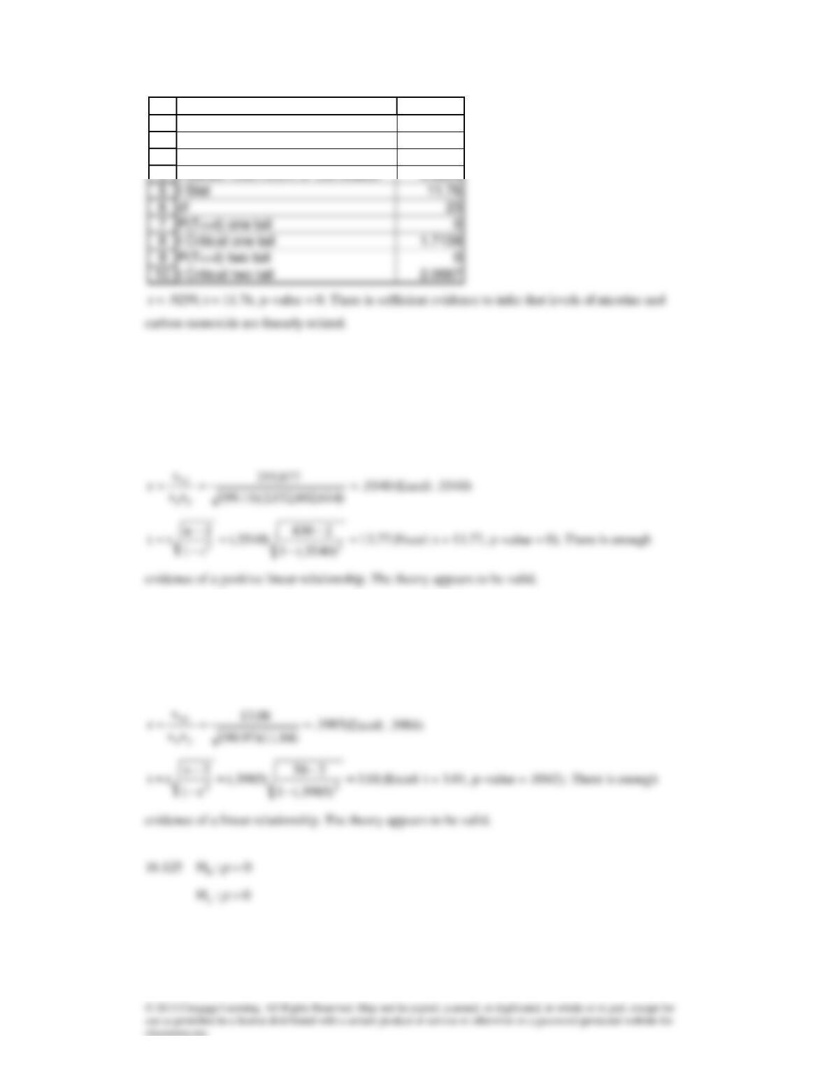
Correlation
Tar and Nicotine
Pearson Coefficient of Correlation 0.9766
t Stat 21.78
16.123
0:H0=
0:H1
Rejection region:
645.1ttt 428,05.2n, == −
or
16.124
0:H0=
0:H1
Rejection region:
009.2ttt 48,025.2n,2/ = −
or
009.2ttt 48,025.2n,2/ −=−=− −
0:H0=
1
2
3
4
A B
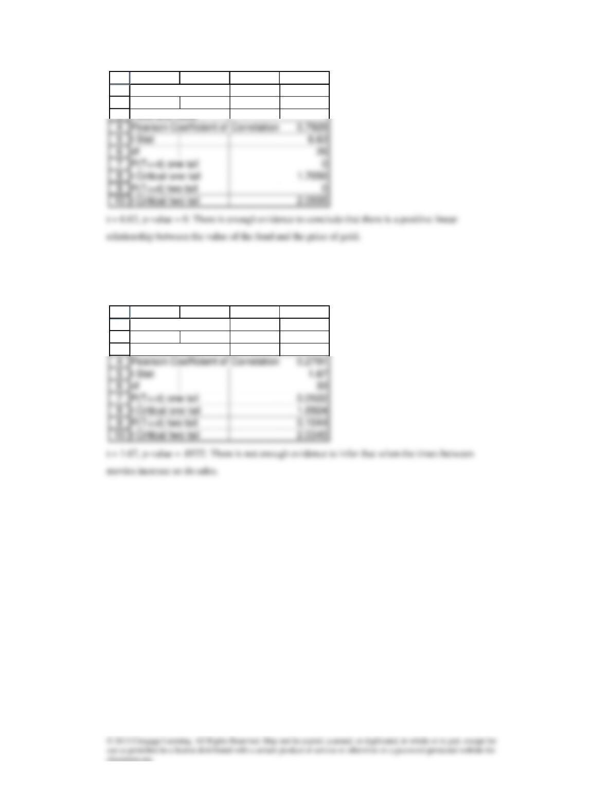
Correlation
Nicotine and CO
Pearson Coefficient of Correlation 0.9259
16.126
0:H0=
0:H1
1
2
3
A B C D
Correlation
Fund and Gold
1
2
3
A B C D
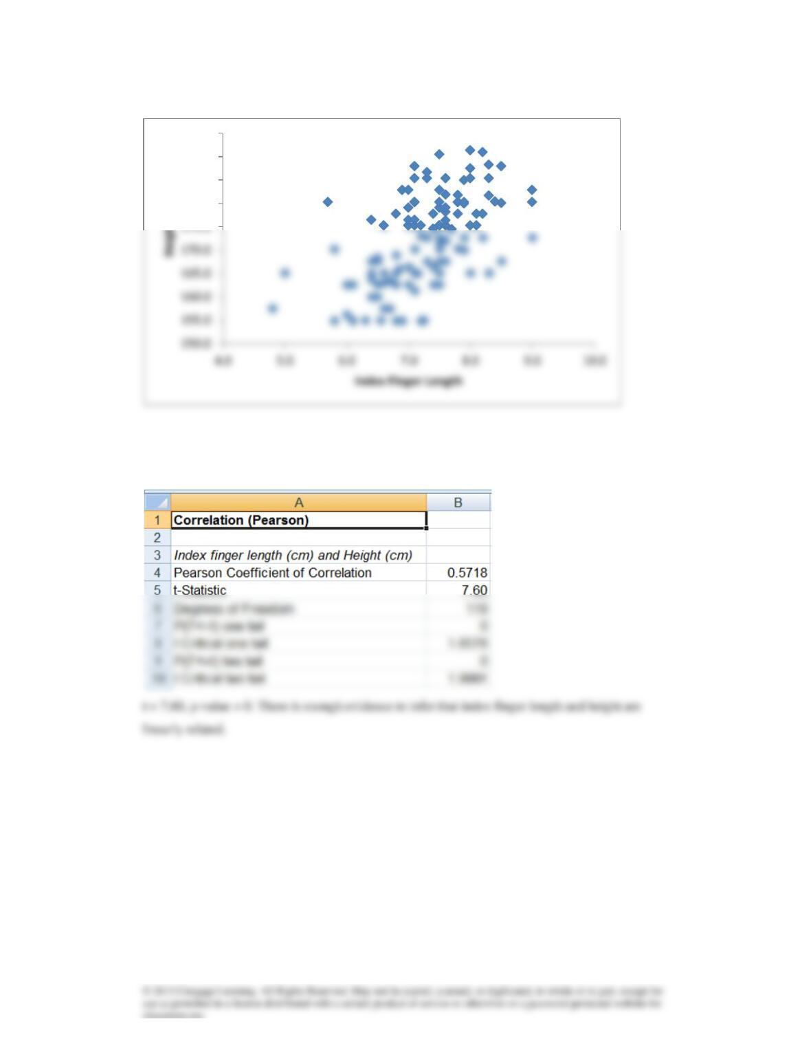
Correlation
Time and Sales
16.127 a
b.
0:H0=
0:H1
180.0
185.0
190.0
195.0
c.
16.128
0:H0=
0:H1
16.129
0:H0=
0:H1
1
2
3
4
A B
Correlation
Hours and GPA
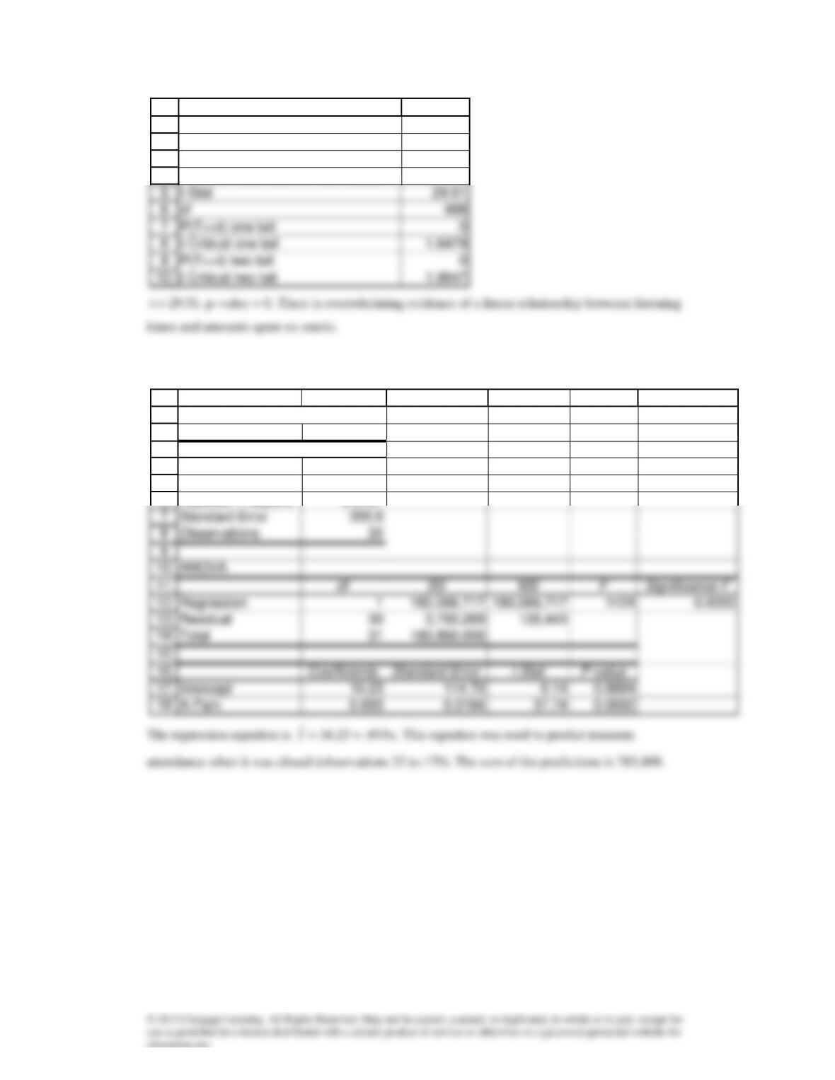
Pearson Coefficient of Correlation -0.5748
Case 16.1 a
8
1
2
3
4
A B
Correlation
Times and Amount
Pearson Coefficient of Correlation 0.7976
1
2
3
4
5
6
A B C D E F
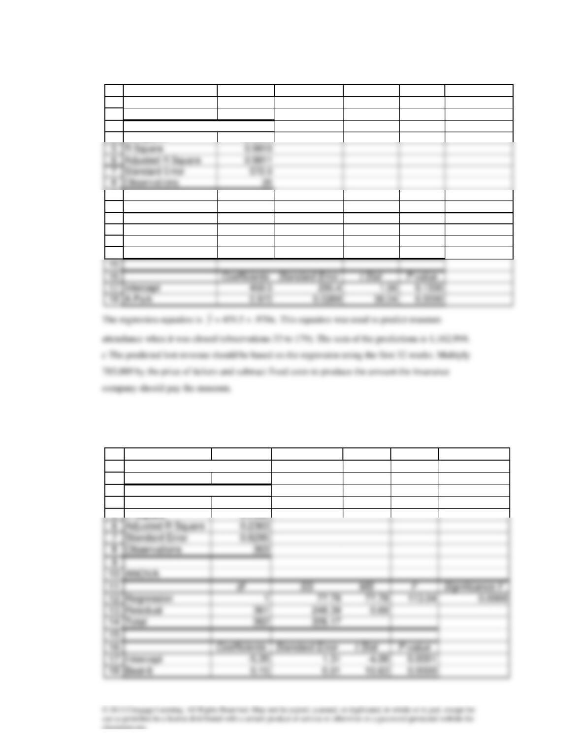
SUMMARY OUTPUT
Regression Statistics
Multiple R 0.9896
R Square 0.9794
Adjusted R Square 0.9787
b
15
Case 16.2
Regression using the best 6 OACs:
1
2
8
3
4
9
10
11
12
13
14
A B C D E F
SUMMARY OUTPUT
Regression Statistics
Multiple R 0.9909
ANOVA
df SS MS F Significance F
Regression 1 426,295,375 426,295,375 1299 0.0000
Residual 24 7,875,875 328,161
Total 25 434,171,250
1
2
3
4
A B C D E F
SUMMARY OUTPUT
Regression Statistics
Multiple R 0.4883
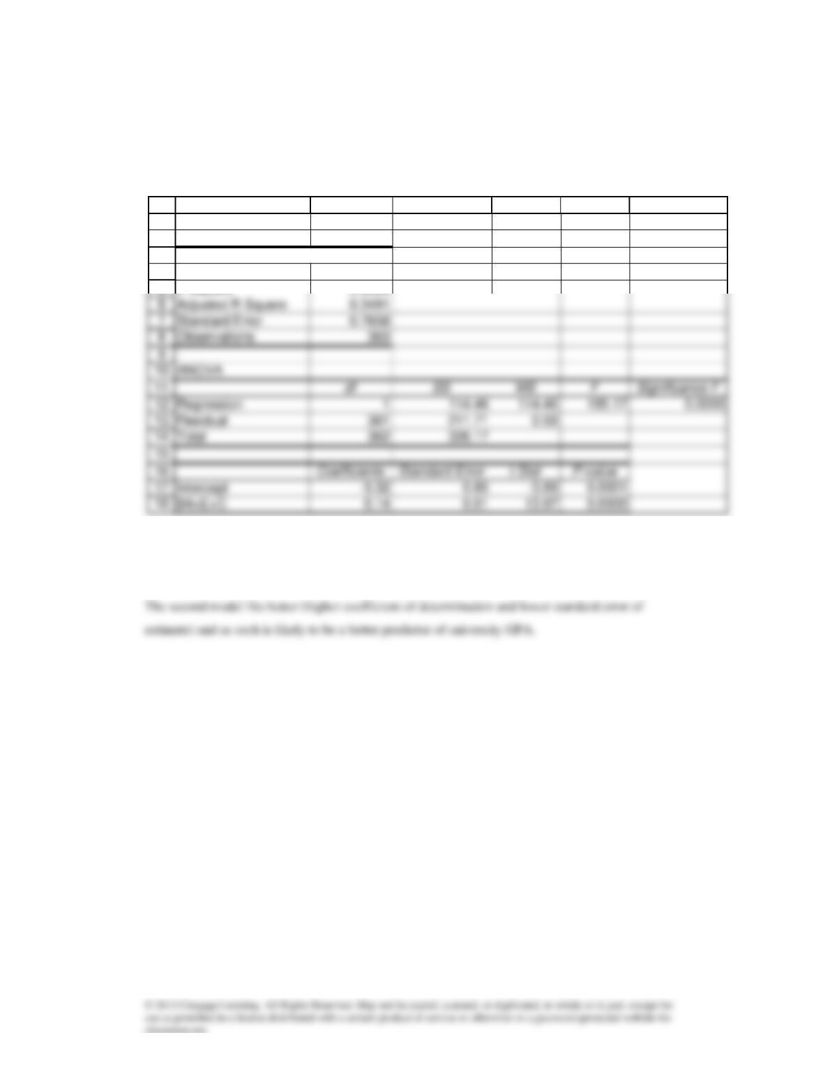
t = 10.63, p–value = 0. There is evidence of a linear relationship between the average of the best 6
OACs and university GPA.
2
R
= .2385,
s
= .8295
Regression using the best 4 OACs plus English and calculus:
8
t = 13.97, p–value = 0; there is evidence of a linear relationship between the average of the best 4
OACs plus English and calculus and university GPA.
2
R
= .3509,
s
= .7658.
1
2
3
4
5
A B C D E F
SUMMARY OUTPUT
Regression Statistics
Multiple R 0.5924
R Square 0.3509