Unlock document.
This document is partially blurred.
Unlock all pages and 1 million more documents.
Get Access

Because the subject of labor demand was extensively treated in Chapter 11, the problems in this
chapter focus primarily on labor supply and on equilibrium in the labor market. Most of the labor
supply problems (16.1–16.3) start with the specification of a utility function and then ask
students to explore the labor supply behavior implied by the function. The primary focus of most
of the problems that concern labor market equilibrium is on monopsony and the marginal
expense concept (problems 16.5–16.7). Analytical problems are concerned with generalizing the
labor supply problems to consider risk, family labor supply, and intertemporal labor supply.
Comments on Problems
16.1 This problem is an algebraic example of labor supply that is based on a Cobb−Douglas
(constant budget shares) utility function. Part (b) shows in a simple context the work
disincentive effects of a lump-sum transfer. Three-fourths of the extra 4,000 is “spent” on
leisure which, at a price of $5 per hour, implies a 600-hour reduction in labor supply. Part
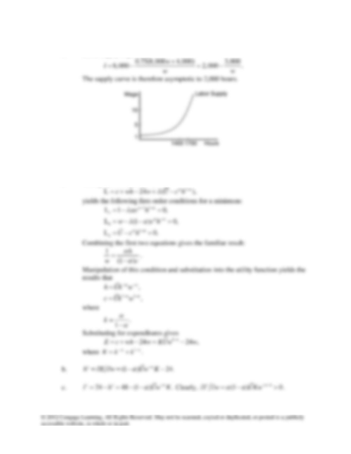
(c) then illustrates a positive labor supply response to a higher wage since the $3,000
spent on leisure will now only buy 300 hours. Notice that a change in the wage would not
affect the solution to part (a), because, in the absence of nonlabor income, the constant
share assumption assures that the individual will always choose to consume 6,000 hours
(=3/4 of 8,000) of leisure.
16.2 This problem uses the expenditure function approach to study labor supply. It shows why
income and substitution effects are precisely off-setting in the Cobb–Douglas case.
16.3 This problem is an application of labor supply theory to the case of means-tested income
transfer programs. The problem results in a kinked budget constraint. Reducing the
implicit tax rate on earnings (parts (f) and (g)) has an ambiguous effect on H since
income and substitution effects work in opposite directions.
16.4 This problem is a simple supply–demand example that asks students to compute various
equilibrium outcomes.
16.5 This problem is an illustration of marginal expense calculation. The problem also shows
that imposition of a minimum wage may actually raise employment in the monopsony
case.
16.6 This problem is an example of monopsonistic discrimination in hiring. The problem
shows that wages are lower for the less elastic supplier. The calculations are relatively
simple if students calculate marginal expense correctly.
CHAPTER 16:
Labor Markets

Chapter 16: Labor Markets
185
16.7 This is a bilateral monopoly problem for an input (here, pelts). Students may get confused
on what is required here, so they should be encouraged first to take an a priori graphical
approach and then try to add numbers to their graph. In that way, they can identify the
relevant intersections that require numerical solutions.
16.8 This problem is a numerical example of the union–employer game illustrated in Example
16.5.
Analytical Problems
16.9 Compensating wage differentials for risk. This problem develops the idea of a
certainty-equivalent wage rate.
16.10 Family labor supply. This problem introduces (in part (b)) the concept of “home
production.” The functional forms specified here are so general that this problem should
be regarded primarily as a descriptive one that provides students with a general
framework for discussing various possibilities.
16.11 A few results from demand theory. This problem shows how many problems in labor
supply theory can be addressed using demand theory concepts from Part 2 of the text.
16.12 Intertemporal labor supply. This problem is an introduction to some general concepts
in the theory of multiperiod labor supply. Because time has not yet been explicitly
introduced, however, the results pertain only to a situation with no discounting.
Solutions
c. With the higher wage, full income is $84,000, $63,000 of which will be devoted
Chapter 16: Labor Markets
186
d. Labor supply is given by
16.2
a. Setting up the Lagrangian,
Chapter 16: Labor Markets
187
d. The algebra is considerably simplified here by assuming
0.5, 2K
==
and using
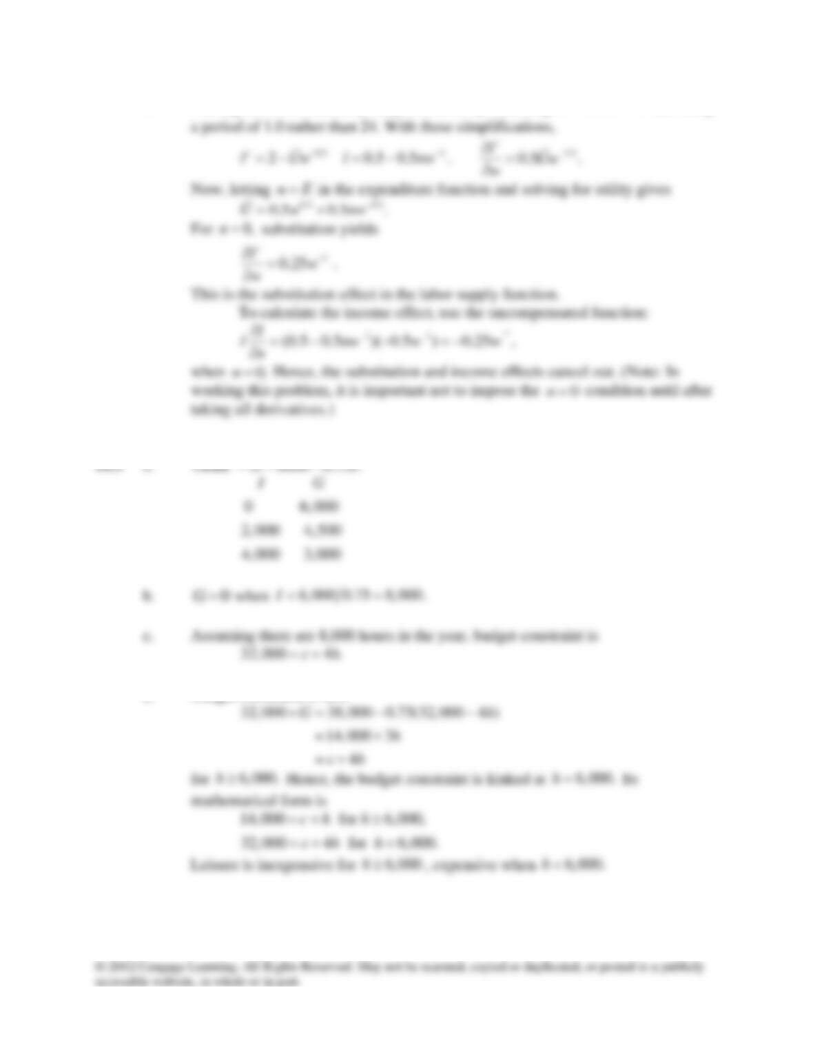
d. Budget constraint is now
Chapter 16: Labor Markets
188
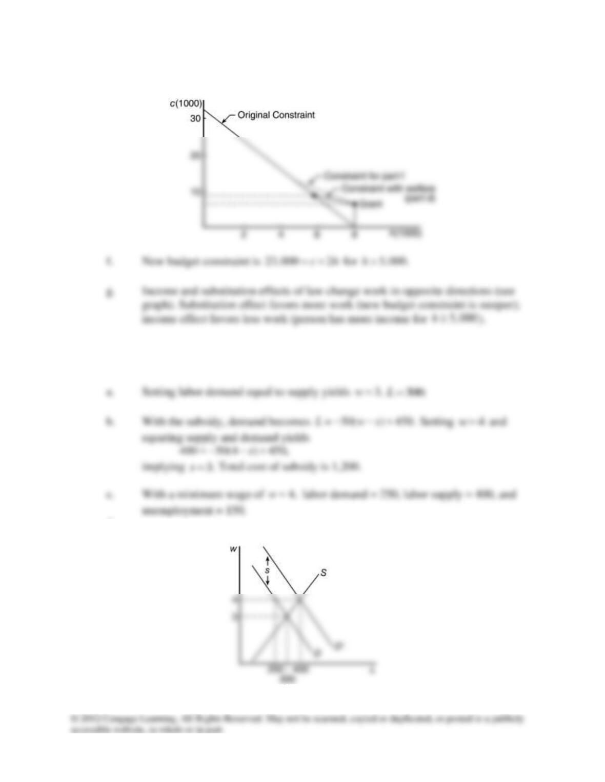
e.
16.4 Labor demand is
50 450,Lw= − +
and labor supply is
100 .Lw=
d.
Chapter 16: Labor Markets
189
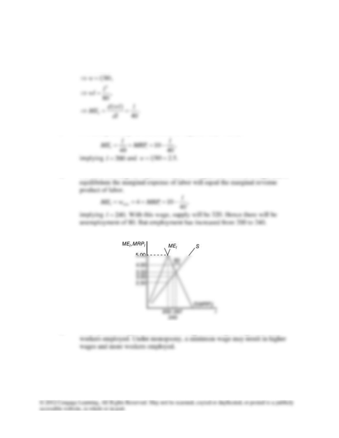
16.5 Given the supply curve for labor, marginal expense is computed as
80 ,
lw
=
a. For monopsonist, profit maximization required
ll
ME MRP=
:
b. For Carl, the marginal expense of labor now equals the minimum wage, and in
c.
d. Under perfect competition, a minimum wage means higher wages but fewer
16.6 First, look at the case of males:
Chapter 16: Labor Markets
190
b. From Dan’s perspective, demand for pelts equals
1,200 20 .
xx
MRP x p= − =
Chapter 16: Labor Markets
191
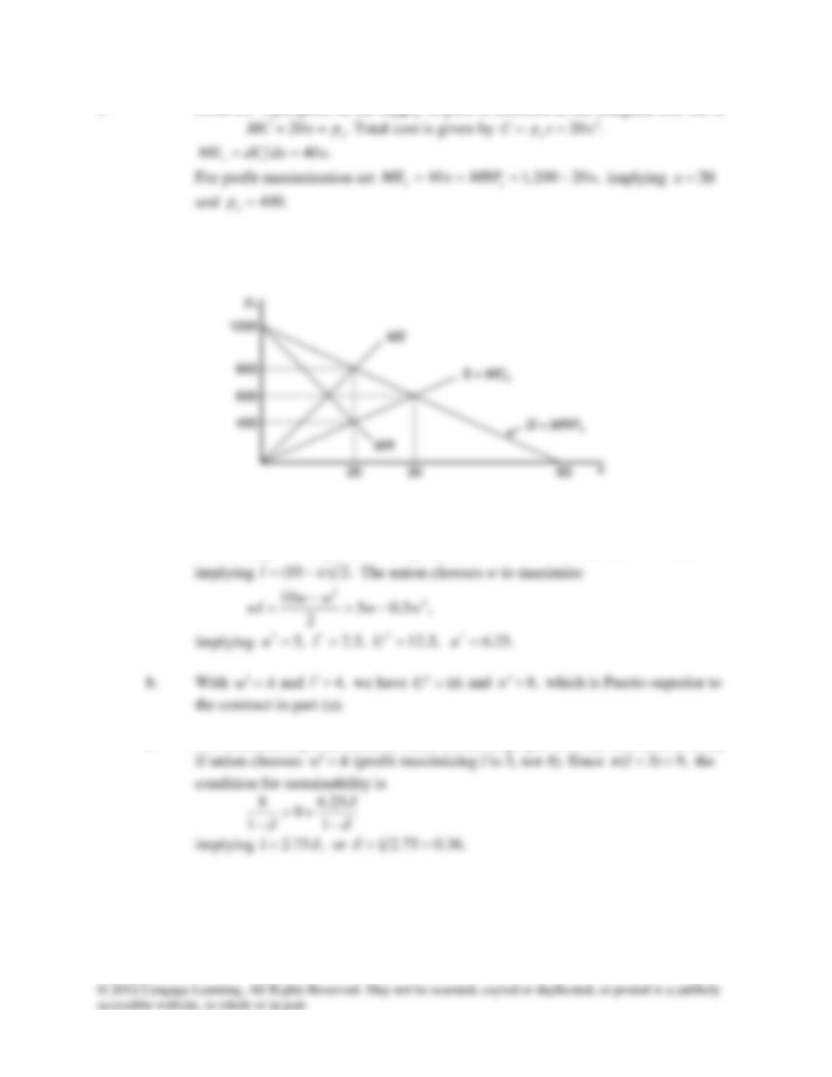
c. From UF’s perspective, the supply of pelts is reflected in the marginal cost curve
d. Both the monopolist and monopsonist agree on
20,x=
but they differ widely on
price to be paid (800 vs. 400). Bargaining will determine the result.
16.8 a. As in Example 16.5, this is solved by backward induction. In the
second stage of the game, the employer chooses l to maximize
2
10 ,l l wl−−
c. For sustainability, one needs to focus on the employer who has incentive to cheat
Chapter 16: Labor Markets
192
Analytical Problems
16.9 Compensating wage differentials for risk
Considering the first (riskless) job,
2
( ) 100 0.5U y y y=−
and
y wl=
with
5w=
and
16.10 Family labor supply
16.11 A few results from demand theory
a. Applying the envelope theorem to Equation 16.20,
Chapter 16: Labor Markets
193
b. Using the logic of the development of the Slutsky equation, for any consumption
good
c. Marginal expense is the change in total labor costs for a change in hiring:
,lw
l
,,
lw
l
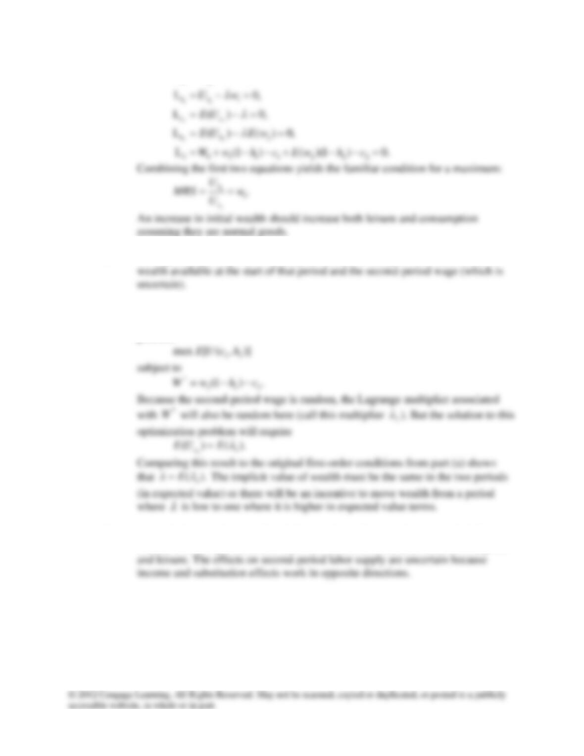
16.12 Intertemporal labor supply
a. The Lagrangian expression for this utility-maximization problem is
Chapter 16: Labor Markets
194
0,
cc
U
= − =
L
b. The equation just says that second-period indirect utility is a function of the
c. Because V is an optimized function we need to return to its original Lagrangian
expression to interpret derivatives. The indirect utility function arises from the
problem
wealth. The first-period effects therefore should be to increase both consumption


