Table 16.6a: Numerical solution of modal equations by the linear acceleration method
i
t 1
q 2
q 1
u 2
u 3
u 4
u 5
u
0.05 –0.0258 –0.0258 –0.0151 –0.0250 –0.0278 –0.0254 –0.0225
0.15 –0.6468 –0.6468 –0.3463 –0.5852 –0.6725 –0.6485 –0.6015
0.25 –2.5521 –2.5521 –1.1630 –2.0422 –2.5076 –2.6343 –2.6183
0.35 –5.4643 –5.4643 –2.0958 –3.8562 –5.0872 –5.7875 –6.0807
0.45 –8.1139 –8.1139 –2.7485 –5.2498 –7.2937 –8.7293 –9.4667
0.55 –8.8024 –8.8024 –2.8215 –5.4854 –7.7980 –9.5297 –10.4628
0.65 –6.2820 –6.2820 –1.9414 –3.8202 –5.5136 –6.8280 –7.5540
0.75 –0.5386 –0.5386 0.0354 –0.0631 –0.3283 –0.6607 –0.8907
0.85 6.9161 6.9161 2.5620 4.7620 6.3739 7.3588 7.8052
0.95 13.4365 13.4365 4.6085 8.7683 12.1191 14.4342 15.6081
1.05 16.2459 16.2459 5.3255 10.2788 14.4767 17.5442 19.1683
1.15 14.1444 14.1444 4.6237 8.9322 12.5948 15.2795 16.7043
1.25 7.9895 7.9895 2.7538 5.2315 7.2159 8.5777 9.2644
1.35 –0.1882 –0.1882 0.0184 –0.0142 –0.1104 –0.2331 –0.3184
1.45 –7.8712 –7.8712 –2.7052 –5.1437 –7.1034 –8.4536 –9.1367
1.55 –12.8231 –12.8231 –4.3476 –8.3019 –11.5297 –13.7941 –14.9563
1.65 –13.7320 –13.7320 –4.5140 –8.7046 –12.2455 –14.8247 –16.1870
1.75 –10.5473 –10.5473 –3.4646 –6.6826 –9.4038 –11.3875 –12.4360
1.85 –4.4269 –4.4269 –1.5395 –2.9166 –4.0081 –4.7478 –5.1169
1.95 2.6686 2.6686 0.8445 1.6488 2.3564 2.8932 3.1851
14
Table P16.6b
i
t )1.0Δ(
5tu )05.0Δ(
5tu 5
u
(Theoretical)
0.10 –0.1742 –0.1795 –0.1804
0.30 –4.0229 –4.2287 –4.2998
0.50 –10.0877 –10.3933 –10.4925
0.70 –4.7301 –4.6169 –4.5850
0.90 11.3579 12.0331 12.2796
1.10 18.2966 18.6839 18.7924
1.30 5.1327 4.5446 4.3529
1.50 –11.6901 –12.5380 –12.8543
1.70 –14.9016 –14.8880 –14.8285
1.90 –2.0069 –0.9202 –0.5740
15
Problem 16.7
a language of your choice using a time step of 0.05 sec.
Solution:
The 55 mass, damping, and initial stiffness matrices
1.0 Initial calculations.
1.1 Since the system starts from rest, 0uu
00 ;
therefore,
0f
0
S.
087.0137.0339.0981.15.110
1.6 Substituting m, c, and tΔin step 1.6 in Table
16.3.1 gives
545.228.97
224.0427.0118.206.97
1
2.0 Calculations for each time step i.
16
Table P16.7: Numerical solution by the central difference method
i
t 1
u 2
u 3
u 4
u 5
u
0.05 0.0000 0.0000 0.0000 0.0000 0.0000
0.15 –0.4208 –0.5618 –0.5702 –0.5727 –0.5735
0.25 –1.2518 –2.0406 –2.4520 –2.5954 –2.6128
0.35 –2.5784 –3.8765 –5.0819 –5.8396 –6.2157
0.45 –4.8851 –6.5821 –7.8163 –8.9214 –9.6809
0.55 –6.8531 –9.3900 –10.3592 –10.9546 –11.1065
0.65 –7.2581 –10.0618 –10.7194 –10.9997 –11.1181
0.75 –5.5877 –7.4676 –8.1300 –8.7881 –9.1320
0.85 –3.8460 –4.2993 –3.8473 –3.9174 –4.1022
0.95 –1.1925 –1.4014 0.0688 1.6356 2.5320
1.05 1.7963 2.1930 4.0292 6.0310 6.4831
1.15 4.1607 5.7289 7.0520 8.1679 8.2798
1.25 5.7262 7.0683 8.5265 9.3454 9.4638
1.35 5.4096 7.0208 8.5179 9.7603 10.2484
1.45 4.9397 6.1701 7.6325 9.3028 9.5438
1.55 4.7642 5.6994 6.4835 7.3875 7.5490
1.65 4.2730 4.6411 5.1459 5.4529 5.1979
1.75 3.6118 3.2808 3.4723 3.9072 3.8311
1.85 3.0881 2.7373 2.7534 3.0641 2.9156
1.95 3.3270 2.9803 2.9176 3.0997 2.7192

17
Problem 16.8
Solve the problem in Example 16.2, implemented by a
computer program in a language of your choice.
Solution:
Problem 16.9
Solve Problem 16.8 with a uniform distribution of lateral
forces.
Solution:
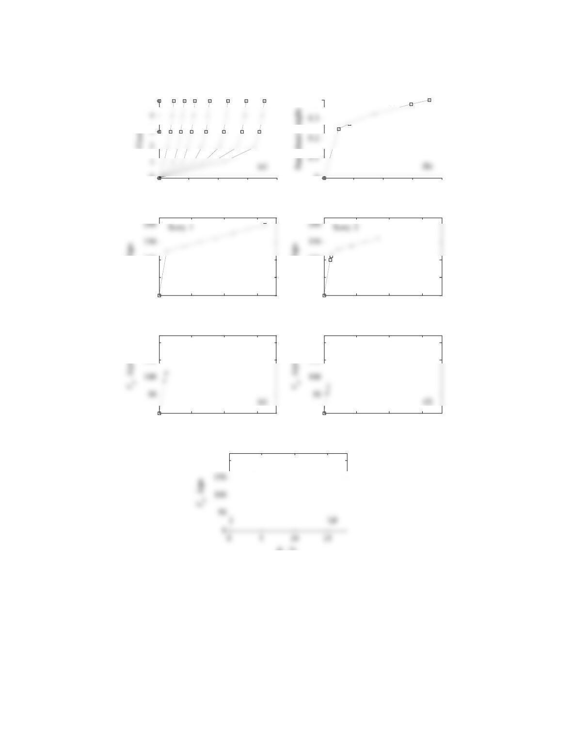
Steps 1.0 to 4.0 of the procedure of Table 16.3.2 are
P16.9b. Story shear–story drift relationships are presented
in Figs. E16.9c–g for the five stories of the building.
Table P16.9: Results of nonlinear static analysis for a
uniform distribution of lateral forces
i
1
u 2
u 3
u 4
u 5
u
0 0.00 0.00 0.00 0.00 0.00
1.1 3.75 4.85 5.68 6.23 6.50
1.3 8.75 11.00 11.98 12.63 12.95
1.5 13.75 20.00 21.13 21.88 22.25
19
01234
0
5
Disp lacement/height, %
= 0 1 1.11.2 1.3 1.4 1.5 1.6
01234
0
0.4
Displacement/height, %
0 5 10 15
0
50
100
1 , in.
V1 , kips
(c)
0 5 10 15
0
50
100
2 , in.
V2 , kips
(d)
0 5 10 15
0
150
200
3 , in.
Story 3
0 5 10 15
0
150
200
4 , in.
Story 4
200
5 , in.
Story 5
Figure P16.9
20
Problem 16.10
Solve the problem in Example 16.3, implemented by a
computer program in a language of your choice.
Solution:
Solution to this problem is available as Example 16.3
in the textbook.
21
Problem 16.11
Solve the problem in Example 16.4, implemented by a
computer program in a language of your choice.
Solution:
Solution to this problem is available as Example 16.4
in the textbook.
Problem 16.12
Solve the problem in Example 16.4 using modified
Newton–Raphson iteration. Compare the number of
iterations required for convergence using Newton–
Raphson iteration (Problem 16.11) and modified Newton–
Raphson iteration (Problem 16.12).
Solution:
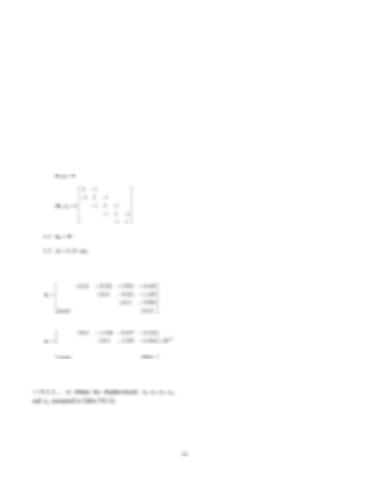
The 55 mass, damping and initial stiffness matrices
were defined in Example 16.4. We now implement the
procedure of Table 16.3.3 as follows.
1.0 Initial calculations.
1.1 State determination for 0u
0
1.4 Matrices 1
a and 2
a
175.0274.0679.0962.34.117
2.545110.0
087.0137.0340.0981.15.110
2.0 Calculations for each time step i.
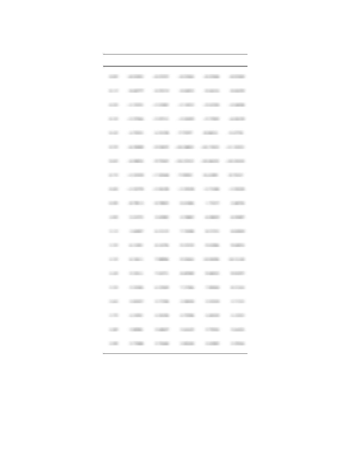
Computational steps 2.0 and 3.0 are implemented for
23
Table P16.12: Numerical solution by constant average
acceleration method with modified Newton–Raphson iteration
i
t 1
u 2
u 3
u 4
u 5
u
0.00 0.0000 0.0000 0.0000 0.0000 0.0000
0.10 –0.1599 –0.2027 –0.2134 –0.2162 –0.2170
0.20 –0.8085 –1.2221 –1.3939 –1.4561 –1.4753
0.30 –1.8010 –2.9592 –3.7088 –4.1001 –4.2559
0.40 –3.5903 –5.1570 –6.4189 –7.3881 –7.8912
0.50 –5.7500 –7.8894 –9.0346 –10.0035 –10.6082
0.60 –6.9909 –9.7228 –10.6480 –11.1123 –11.2668
0.70 –6.4173 –8.8925 –9.6124 –9.9684 –10.0854
0.80 –4.5725 –5.6692 –5.8777 –6.3031 –6.6348
0.90 –2.2746 –2.3902 –1.4073 –0.9122 –0.7441
1.00 0.7791 0.9285 2.6105 4.1492 5.0590
1.10 3.5179 4.4570 6.3342 7.5641 8.0206
1.20 5.4733 7.4444 8.7198 9.2110 9.2146
1.30 6.4583 8.2244 9.3834 9.9268 10.0786
1.40 5.8352 7.4688 8.9357 9.9435 10.2928
1.50 5.2204 6.5992 7.9125 8.7781 9.1911
1.60 5.2974 6.0435 6.6032 6.9179 6.8865
1.70 4.6731 5.2528 5.3892 5.0787 4.7669
1.80 4.0926 3.9866 4.0614 4.0236 3.7778
1.90 3.7094 3.6345 3.5589 3.5522 3.5834
2.00 3.9438 4.0617 4.2047 4.0169 3.6657