Chap. 16 Drilled Shafts: Axial Load Capacity Based on Static Analysis Methods
16.1 Compare the construction methods for driven piles vs. drilled shafts and discuss the impact of
these differences on their axial load capacity.
Solution
Driven pile construction causes major changes in a zone surrounding the pile including:
movement of soil around the pile, changes in density in soil surrounding the pile, changes in soil
Chap. 16 Drilled Shafts: Axial Load Capacity Based on Static Analysis Methods
16.2 Why is it important for drilled shaft contractors to place the concrete soon after drilling the shaft?
What detrimental effects can occur if the contractor waits too long before placing the concrete?
How might this affect the axial load capacity?
Solution
Drilled shaft construction removes soil during the augering process thus lowering the lateral
earth pressure. If the concrete is not placed soon after drilling, caving conditions may be
Chap. 16 Drilled Shafts: Axial Load Capacity Based on Static Analysis Methods
16.3 Some engineers ignore the toe bearing capacity for downward loaded drilled shafts, while others
consider toe bearing as part of the total capacity. Discuss this difference in practice
Solution
The decision to ignore toe bearing capacity for downward loaded drilled shafts depends on the
type of soil encountered at the project site, size of the shaft, and length of the shaft. Cohesive
Chap. 16 Drilled Shafts: Axial Load Capacity Based on Static Analysis Methods
16.4 An office building is to be supported on a series of 700–mm diameter, 12.0 m long drilled shafts
that will be built using the open hole method. The soil profile at this site is as follows:
Depth (m)
Soil Description
Undrained shear
strength, su (kPa)
0–2.2
Stiff clayey silt (ML)
70
2.2–6.1
Stiff silty clay (CL)
85
6.1–11.5
Very stiff sandy clay (CL)
120
11.5–30.0
Very stiff sandy clay (CL)
180
The groundwater table is at a depth of 50 m. No onsite static load test data is available, the soil
conditions are uniform, and the site characterization program was average. Compute the ASD
allowable downward and upward capacities.
Solution
( )( )
9 9 180 kPa 1620 kPa
nu
qs
′= = =
Layer Depth
(m)
Thickness
(m)
su
(kPa) α
fs
(kPa)
As
(m2)
fs As
(kN)
1 0 – 1.5 1.5 – 0 – – 0
2 1.5 – 2.2 0.7 70 0.55 38.5 1.54 59.3
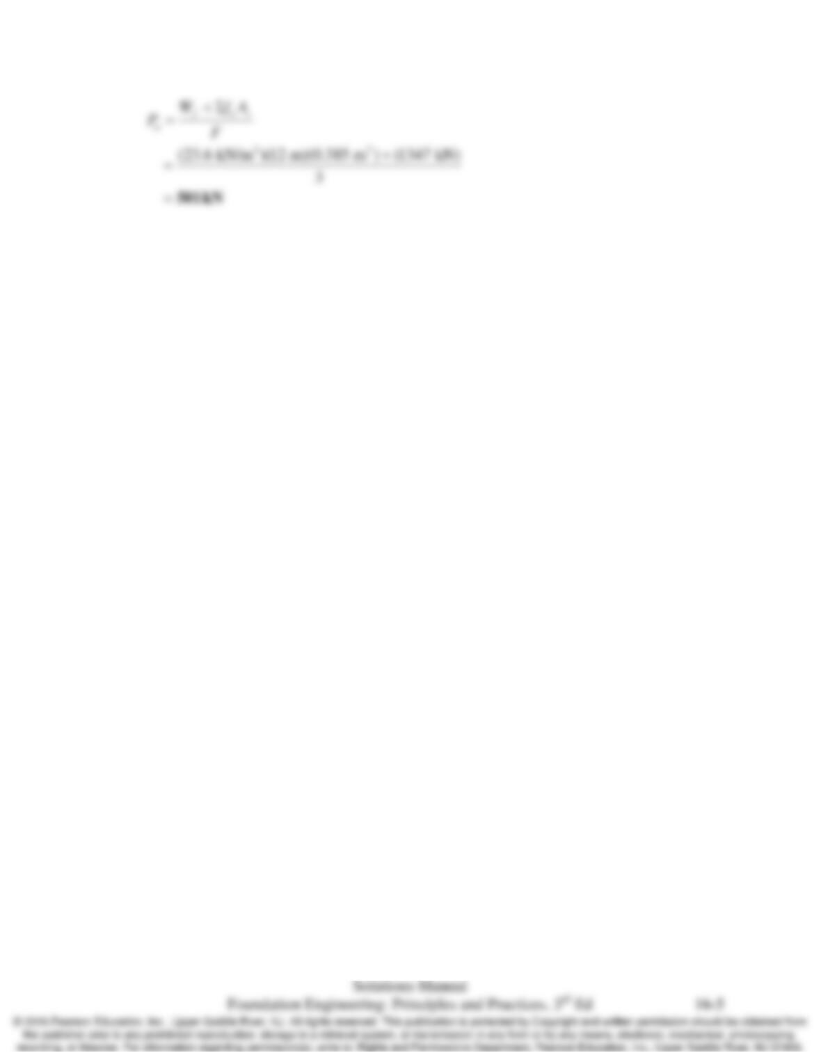
1347
Use F = 3 (per Table 13.2) for no static load test, uniform conditions, and average site
characterization.
=657 kN
Chap. 16 Drilled Shafts: Axial Load Capacity Based on Static Analysis Methods
16.5 Using the data in Problem 16.4 and the AASHTO resistance factors, compute
n
P
φ
and
,up n
P
φ
.
Use a load factor of 0.9 on the weight of the shaft.
Solution
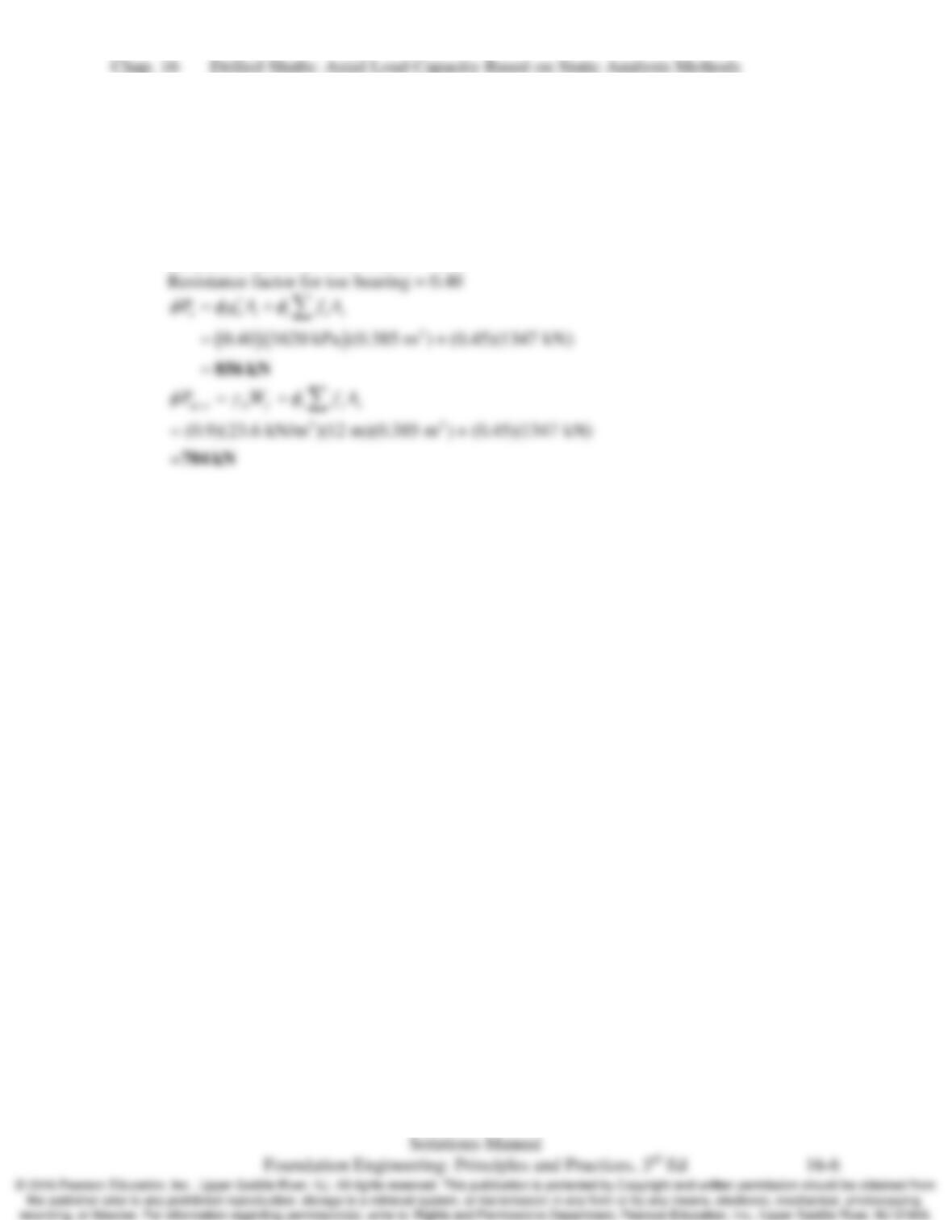
Per Table 13.5, the AASHTO
Resistance factor for side friction = 0.45
Chap. 16 Drilled Shafts: Axial Load Capacity Based on Static Analysis Methods
16.6 A highway bridge pier is to be supported on a single 8 ft diameter 90 ft deep drilled shaft. The
subsurface conditions at this site are:
Depth (ft)
Soil Description
Unit Weight, γ
(lb/ft
3
)
N60
0–15
Silty sand
118
15–42
Sandy silt
115
42–80
Well graded sand
121
80–100
Gravelly sand (30% gravel size)
129
45
The groundwater is at a depth greater than 150 ft. Using the AASHTO resistance factors,
compute
n
P
φ
and
,up n
P
φ
. Use a load factor of 0.9 on the weight of the shaft.
Solution
Side Friction
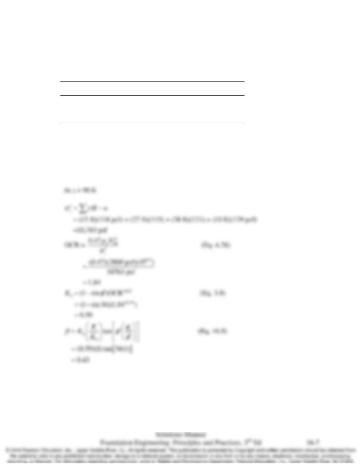
Compute
β
per Brown, et al. (2010):
Chap. 16 Drilled Shafts: Axial Load Capacity Based on Static Analysis Methods
Toe Bearing
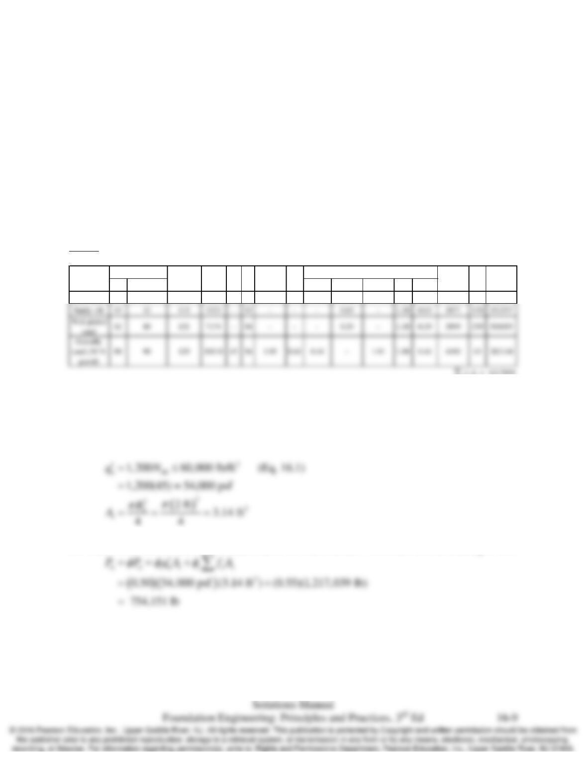
Use Equation 16.1 to compute the net unit toe bearing resistance. Although no N60 values are
44
Per Table 13.5, the AASHTO resistance factor for side friction = 0.55, and for toe bearing is 0.50
Top Bottom Eq 16.9 Eq 16.10 Eq 16.12 Max Design
Silty sand 0 15 118 885 – 35 – – – 0.98 – 1.20 0.98 865 377 326013
(psf)
(ft2)
(lb)
ϒ (lb/ft3)
Soil
Description
Layer Depth (ft)
(psf)
φ
ʹ
OCR
(Eq 4.28)
N60
K0
z
s
′
β
n
f
s
A
ns
fA
Chap. 16 Drilled Shafts: Axial Load Capacity Based on Static Analysis Methods
16.7 Using the soil profile in Problem 16.6, consider an alternative design consisting of a group of 24
inch diameter, 90 ft long drilled shafts. These shafts will be placed 60 inches on center.
(a) Determine the number of shafts required to obtain the same φPn as the single 8 ft diameter
shaft. Draw a plan view sketch of this pile group.
(b) Assume the pile cap will extend 24 inches beyond the edges of the outside piles and will be 3
ft thick. Compute the total volume of reinforced concrete (cap plus shafts) for this alternative,
and compare it with the total volume of reinforced concrete for the single 8 ft diameter shaft
(which does not require a cap).
(c) Discuss these two alternatives.
Solution
Part A
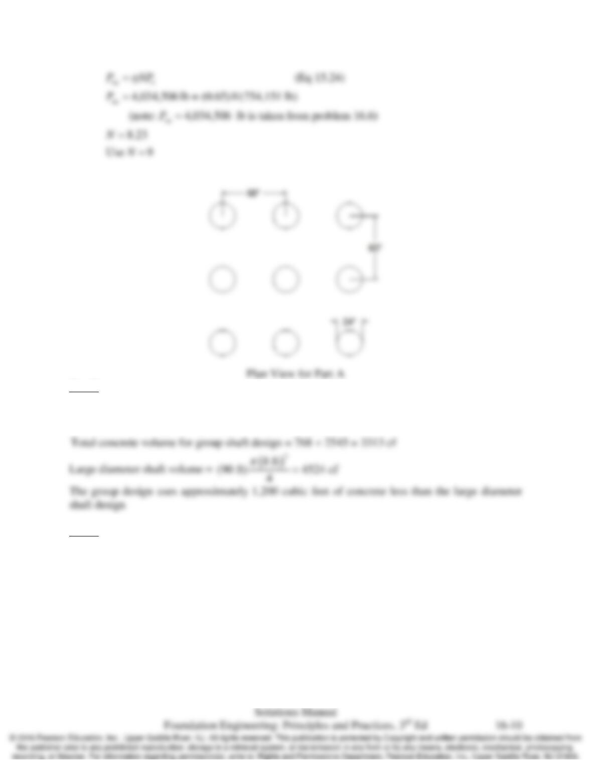
Toe Bearing
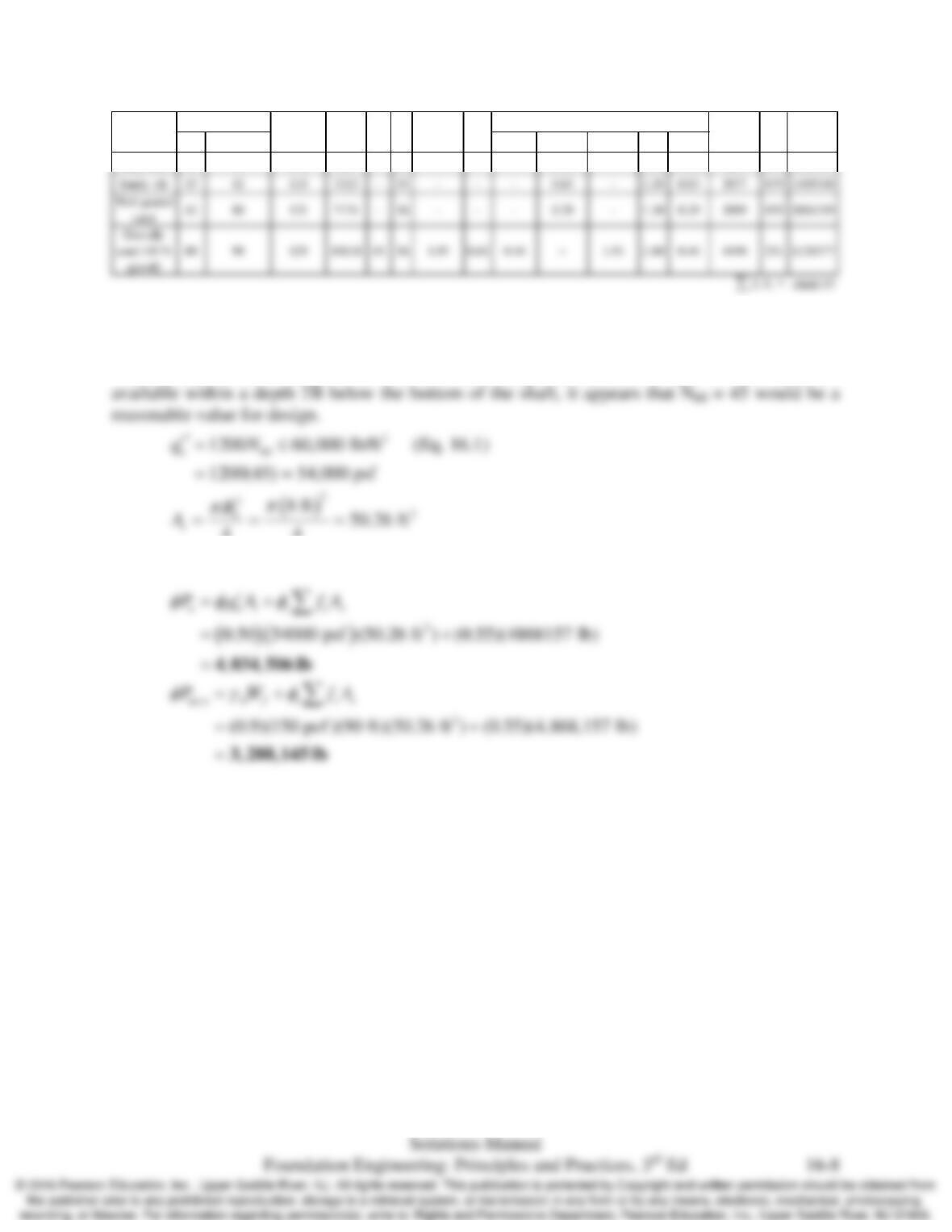
Use Equation 16.1 to compute the net unit toe bearing resistance. Although no N60 values are
available within a depth 2B below the bottom of the shaft, it appears that N60 = 45 would be a
reasonable value for design.
Per Table 13.5, the AASHTO resistance factor for side friction = 0.55, and for toe bearing is 0.50
Top Bottom Eq 16.9 Eq 16.10 Eq 16.12 Max Design
Silty sand 0 15 118 885 – 35 – – – 0.98 – 1.20 0.98 865 94 81503
1217039
(lb)
Soil
Description
Layer Depth (ft)
ϒ (lb/ft
3
)
(psf)
N
60
φ
ʹ
OCR
(Eq 4.28)
K
0
(psf)
(ft
2
)
z
s
′
β
n
f
s
A
ns
fA
ns
fA=
∑
Chap. 16 Drilled Shafts: Axial Load Capacity Based on Static Analysis Methods
Part B
( )
( )
( )
2
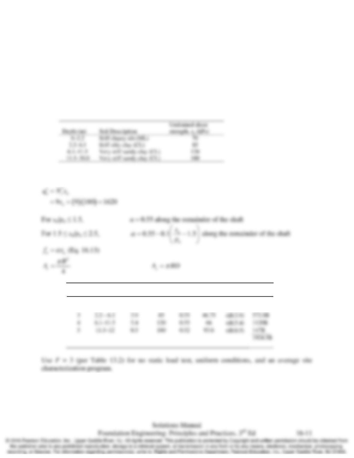
Group shafts volume = 9 shafts 3.14 ft 90 ft = 2545 cf
( )
( )
2
Pile cap volume = 256 ft 3 ft = 768 cf
Part C
Group effects often are not a concern for drilled shafts since drilled shafts typically have larger
diameters. However, drilled shafts also may be used in groups, in which case group effects must
be considered in a fashion similar to that discussed in Section 15.5. However, because of the
difference in construction methods and the associated impacts on the adjacent soils, the group
efficiency factors for drilled shafts are different than those for driven piles. For cohesionless
soils, AASHTO (2012) uses
η
= 0.65 for piles spaced 2.5 diameters on center,1.0 when 4.0 or
more diameters on center, and a linearly interpolated value between these spacings. So long as
good workmanship is used, these values are probably conservative (Brown, et al., 2010). For
cohesive soils, AASHTO (2012) uses
η
= 1, but also requires checking for block failure. Clearly
the group shaft design uses less concrete compared to the large diameter shaft for this scenario.
Chap. 16 Drilled Shafts: Axial Load Capacity Based on Static Analysis Methods
16.8 Using the soil profile in Problem 16.4, determine the required diameter and length needed to
support an ASD design downward load of 550 kN. Note there are many different diameter –
length combinations that would be satisfactory, but select one that you think would be most
appropriate.
Solution:
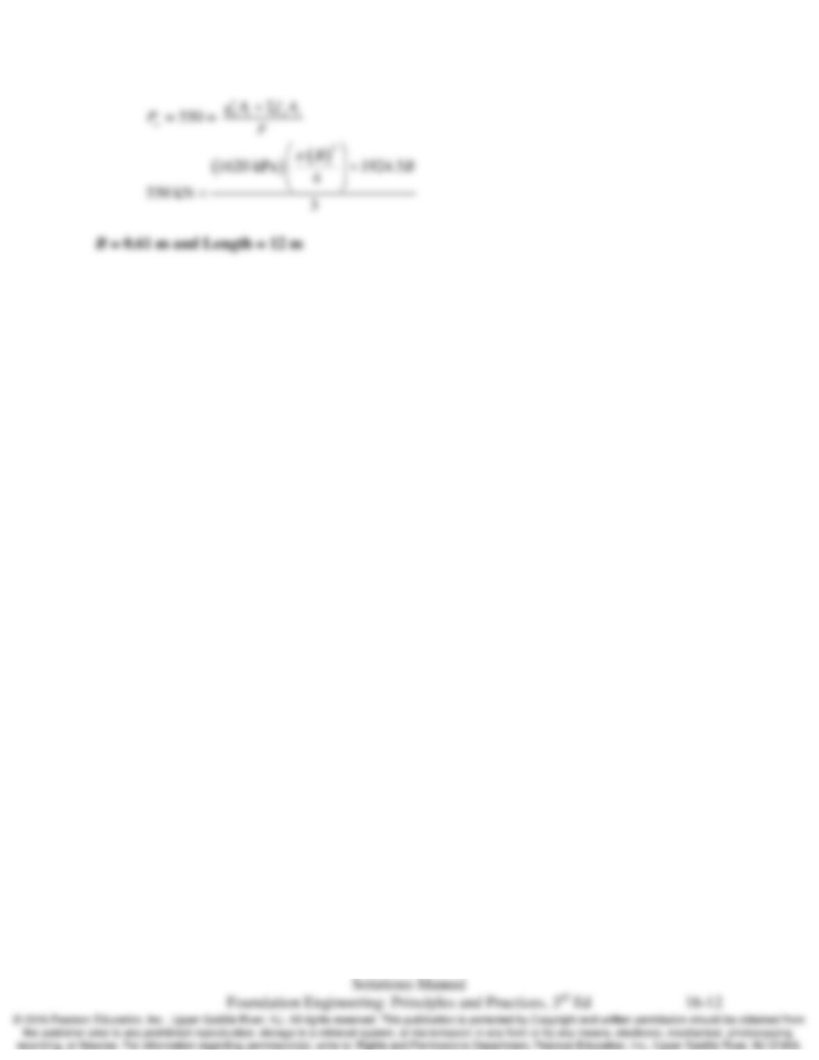
Drilled shafts using the open hole method are being proposed. The soil profile at this site is as
follows:
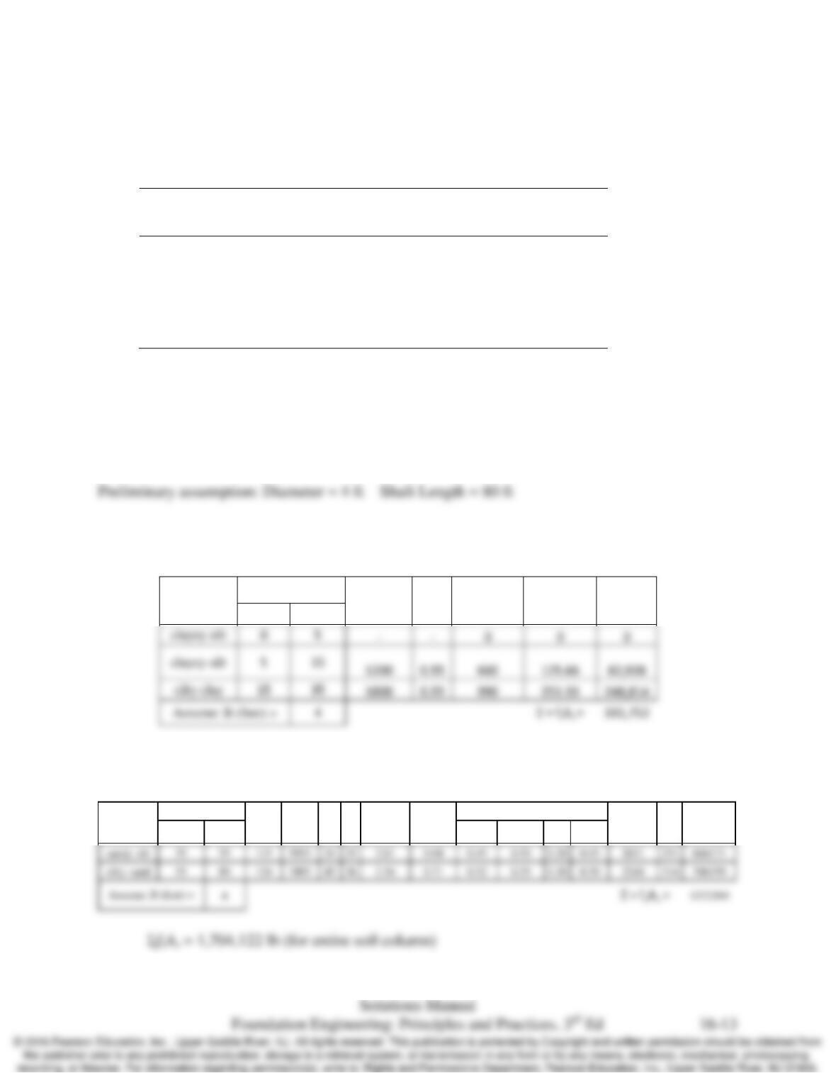
Assume that for D/B > 3 with su ≤ 250 kPa
Layer
Depth
(m)
Thickness
(m)
s
u
(kPa)
α
f
s
(kPa)
A
s
(m
2
)
f
s
A
s
(kN)
1
0 – 1.5
1.5
–
0
–
–
0
2
1.5 – 2.2
0.7
70
0.55
38.5
πB(0.7)
84.66B
3
2.2 – 6.1
3.9
85
0.55
πB(3.9)
572.8B
4
5.4
0.55
πB(5.4)
Chap. 16 Drilled Shafts: Axial Load Capacity Based on Static Analysis Methods
Chap. 16 Drilled Shafts: Axial Load Capacity Based on Static Analysis Methods
16.9 A drilled shaft designed in accordance with the AASHTO code must support the following
downward and uplift axial design loads: Pu = 850 k, Pup,u = 270 k. The soil profile consists of:
Depth (ft)
Soil Description
Unit Weight, γ
(lb/ft
3
)
Undrained shear
strength, su
(lb/ft
2
)
N60
0–15 Clayey silt 115 1200
15–35 Silty clay 112 1800
35–55 Sandy silt
(nonplastic) 115 24
55–80 Silty sand 124 43
The groundwater is at a depth of 50 ft. Using the AASHTO resistance factors, select a diameter
and depth for a single drilled shaft to support these design loads. Use a load factor of 0.9 on the
weight of the shaft. Note there are many different diameter – length combinations that would be
satisfactory, but select one that you think would be most appropriate.
Solution
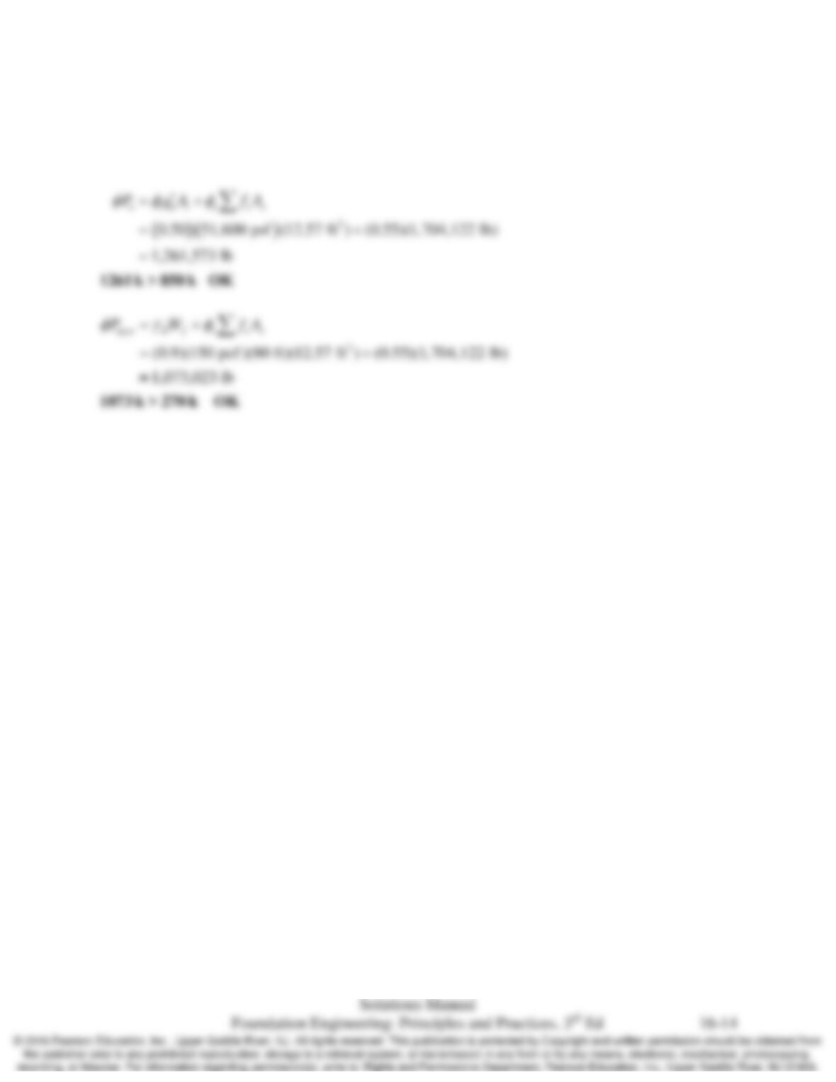
Side Friction for cohesive soils (0 – 35’)
For su/pa ≤ 1.5, α = 0.55 along the remainder of the shaft
Soil
Description
Layer Depth (ft) su (lb/ft2) α
(Eq.16.13)
fs = Suα As (ft2) fsAs
(lb)
Top Bottom
Side Friction for cohesionless soils (35’ – 80’) (must take into account groundwater at 50 ft)
Top Bottom Eq 16.9 Eq 16.10 Max Design
(Eq 4.28)
OCR
(Eq. 3.8)
K
0
β
(Eq. 16.8)
f
s
(psf)
(ft
2
)
f
s
A
s
(lb)
φ
ʹ
Soil
Description
Layer Depth (ft)
ϒ
(lb/ft
3
)
(psf)
N
60
z
s
′
s
A
Chap. 16 Drilled Shafts: Axial Load Capacity Based on Static Analysis Methods
Toe Bearing
2
60
22
1,200 60,000 lb/ft
= 1,200(43) = 51,600 lb/ft 60,000 lb/ft
n
qN
′= ≤
≤
(Eq. 16.1 English)
Chap. 16 Drilled Shafts: Axial Load Capacity Based on Static Analysis Methods
16.10 A full–scale load test has been conducted on a 24–in diameter, 40–ft long instrumented drilled
shaft similar to the one shown in Figure 14.10. The test crew maintained records of the load-
settlement data and the forces in each of the five load cells. The applied load at failure (using
Davisson’s method as described in Chapter 14) was 739,600 lb. The corresponding forces in the
load cells were as follows:
Load Cell
Number Depth
(ft) Force
(lb)
1 3.0 719,360
2 12.0 636,120
3 21.0 487,500
4 30.0 304,320
5 39.0 135,400
There are two soil strata at the site: the first extends from the ground surface to a depth of 15 ft
and has a unit weight of 117 lb/ft3; the second extends from 15 ft to 60 ft and has a unit weight of
120 lb/ft3 above the groundwater table and 127 lb/ft3 below. The groundwater table is at a depth
of 17 ft. Compute the average β factor in each of the two soil strata, and the net unit toe–bearing
resistance,
n
q′
.
Note: Once these site–specific β and
n
q′
values have been computed, they could be used to design
shafts of other diameters or lengths at this site.
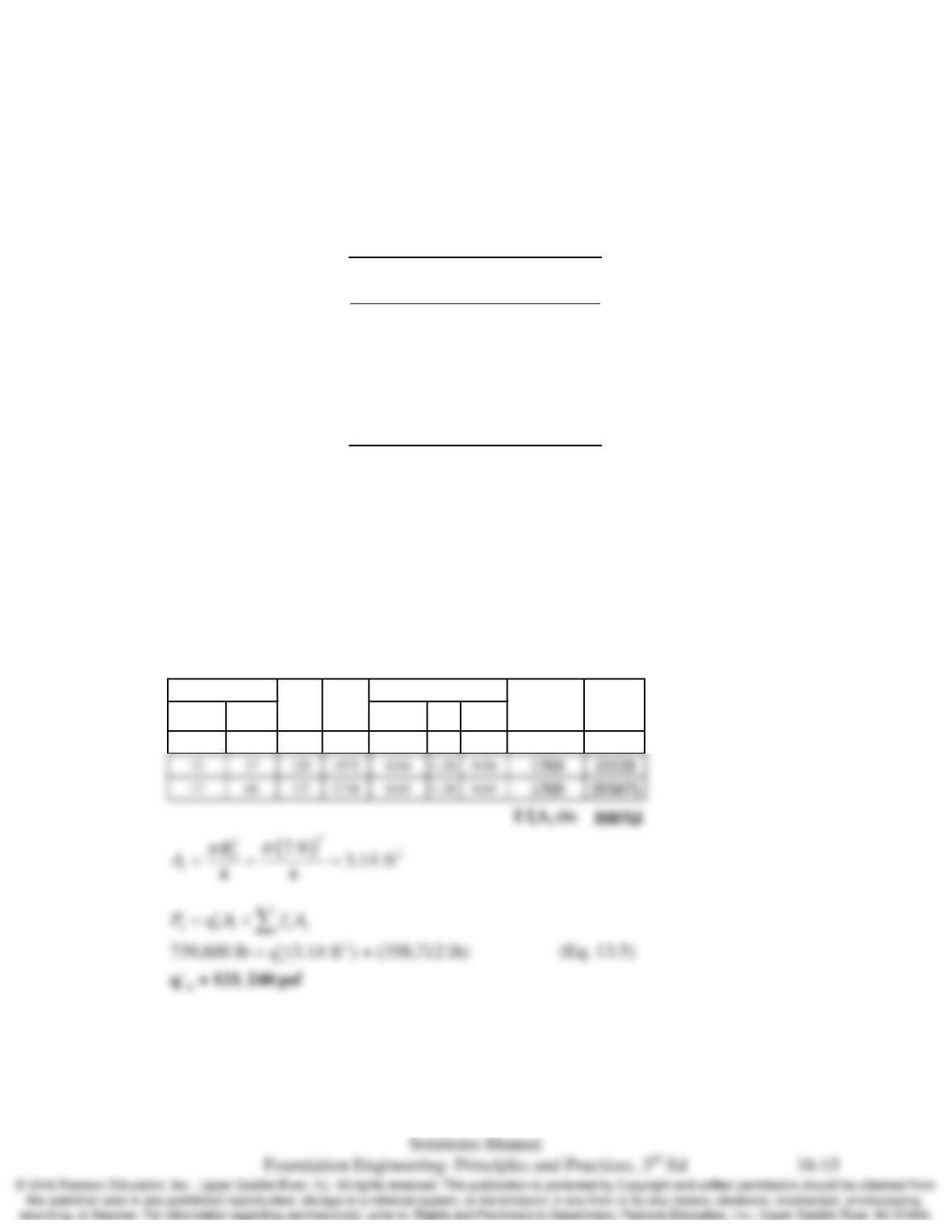
Solution
Top Bottom Eq 16.10 Max Design
0 15 117 877.5 0.98 1.20 0.98
857 80812
β
(Eq. 16.8)
f
s
(psf)
fsAs
(lb)
Layer Depth (ft)
ϒ
(lb/ft
3
)
(psf)
z
s
′