Chap.15 Driven Piles: Axial Load Capacity Based on Static Analysis Methods
15.1 Why would it be inappropriate to design a drilled shaft using a static analysis method developed
for driven piles?
Solution
It would be inappropriate to design a drilled shaft using any analysis designed for a driven pile
for several reasons.
Driven pile installation compacts the soil surrounding the pile. However, a drilled shaft removes
the soil and can also loosen the surrounding soil depending on the installation method used. This
Chap.15 Driven Piles: Axial Load Capacity Based on Static Analysis Methods
15.2 Why would it be inappropriate to use the Terzaghi bearing capacity formulas from Chapter 7 to
determine the toe bearing capacity of a driven pile?
Solution
It would be inappropriate to use Terzaghi’s bearing capacity formulas for driven piles because
driven piles, and all other deep foundations, have different failure mechanisms than what is
Chap.15 Driven Piles: Axial Load Capacity Based on Static Analysis Methods
15.3 An 18 inch diameter closed-end steel pipe pile is to be driven to a depth of 53 ft into the
following soil profile:
Depth (ft) Soil Classification
Unit Weight,
γ
(lb/ft3)
Friction Angle,
φ
′
(deg) OCR
0–5 Silty sand 118 28 5.0
5–20 Fine to medium sand 121 31 3.5
20–50 Silty sand 118 29 2.5
50–60 Well graded sand 123 35 2.0
No predrilling or jetting is to be used. The groundwater table is at a depth of 15 ft. Using a
factor of safety of 3.0, compute the ASD allowable downward load capacity,
a
P
.
Solution
This problem will be separated into three parts: (a) Toe Bearing, (b) Side Friction, and (c)
Determine
a
P
(a) Toe Bearing
Because the soils are primarily cohensionless the following equation will be used to determine
the toe bearing capacity.
From Table 4.7:
0100,000 psf
β
=
Chap.15 Driven Piles: Axial Load Capacity Based on Static Analysis Methods
Next we can calculate r
I
. To do this we must first estimate the Poisson’s ratio using Equation
Now we can find
*
N
γ
and
*
q
N
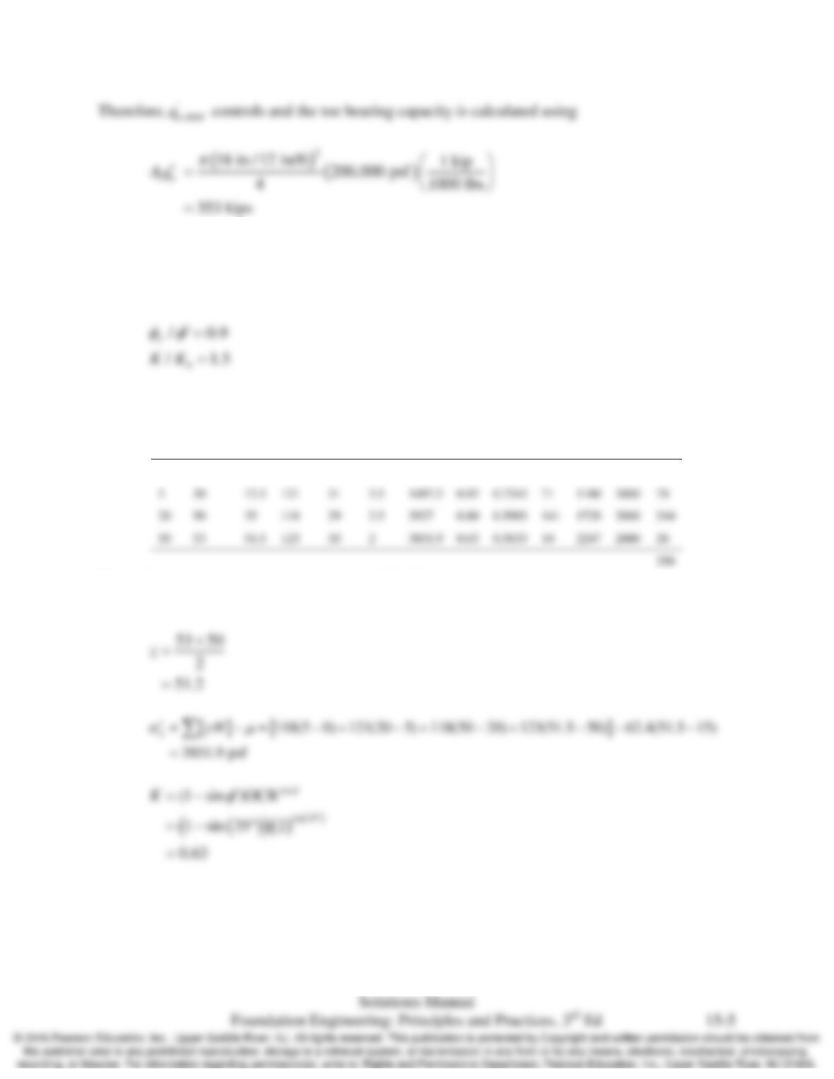
using Figures 15.2 and 15.3 respectively.
Next we can substitute into Equation 15.1 and obtain
n
q′
and find the maximum value of
n
q′
from Table 15.1
Chap.15 Driven Piles: Axial Load Capacity Based on Static Analysis Methods
(b) Side Friction
The first step is to determine values for
/
f
φφ
′
and
0
/KK
from Tables 15.2 and 15.3
respectively.
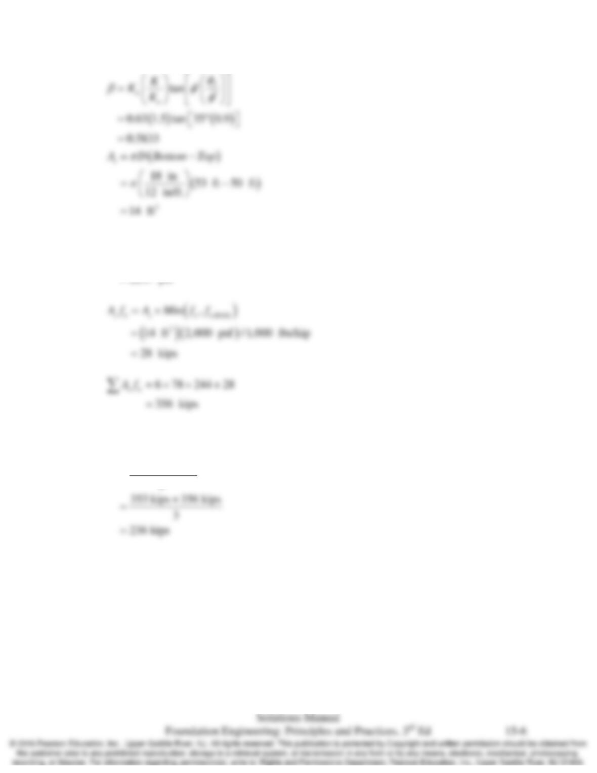
The following table can then needs to be created using the calculations explained below
Top
(ft)
Bottom
(ft)
z
(ft)
γ
(lb/ft3)
φ
‘
(deg) OCR
σz‘
(psf) K0 β
As
(ft2)
fn
(psf)
fn, Max
(psf)
fnAs
(k)
0 5 2.5 118 28 5 295 1.13 0.7972 24 235 2000 6
The following sample calculations use the 50’-53’ layer to demonstrate the formulas required to
obtain the skin friction
Chap.15 Driven Piles: Axial Load Capacity Based on Static Analysis Methods
( )( )
0.5833 3851.9 psf
2247 psf
nz
f
βσ
′
=
=
=
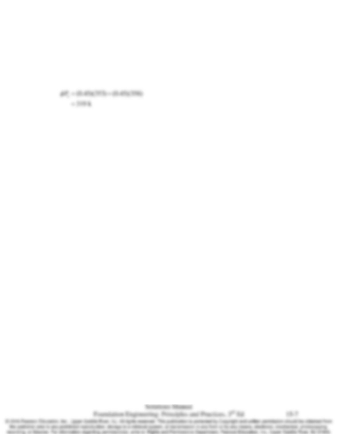
(c) Determine
a
P
nt ns
a
qA fA
PF
′+
=
∑
Chap.15 Driven Piles: Axial Load Capacity Based on Static Analysis Methods
15.4 Using the data in Problem 15.3 and the AASHTO resistance factors, compute
n
P
φ
.
Solution
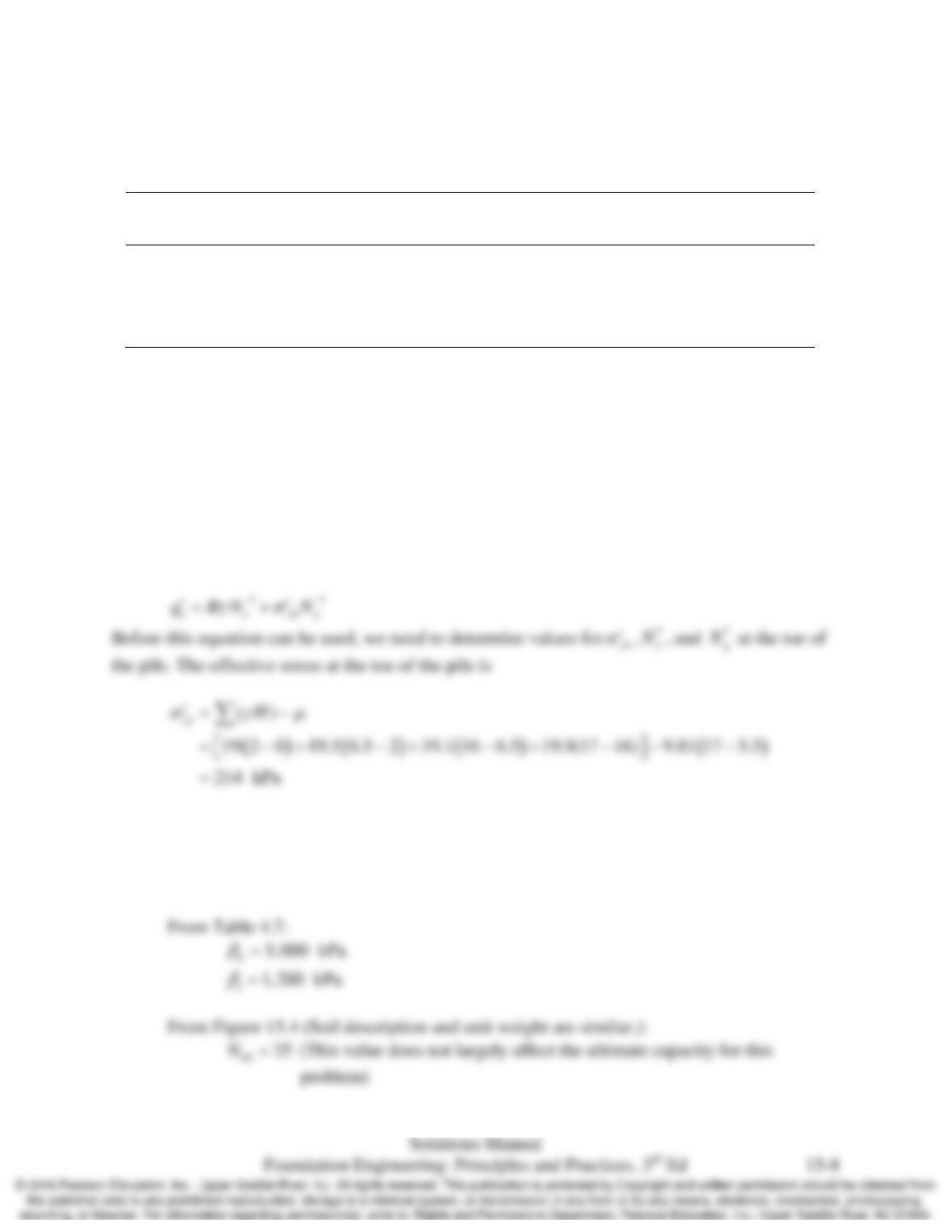
Use
0.45
φ
=
per Table 13.4
Chap.15 Driven Piles: Axial Load Capacity Based on Static Analysis Methods
15.5 A 500 mm diameter closed-end steel pipe pile is to be driven to a depth of 17 m into the
following soil profile:
Depth (m) Soil Classification
Unit Weight,
γ
(kN/m3)
Friction Angle,
φ
′
(deg) OCR
0–2.0 Silty sand 19.0 28 4.5
2.0–6.5 Fine to medium sand 19.5 31 3.5
6.5–16.0 Silty sand 19.1 29 2.5
16.0–17.5 Well graded sand 19.8 35 1.5
No predrilling or jetting is to be used. The groundwater table is at a depth of 5.5 m. Compute the
toe bearing capacity,
nt
qA
′
.
Solution
(a) Toe Bearing
Because the toe bearing soils are cohensionless the following equation will be used to determine
the toe bearing capacity.
To determine
*
N
γ
and
*
q
N
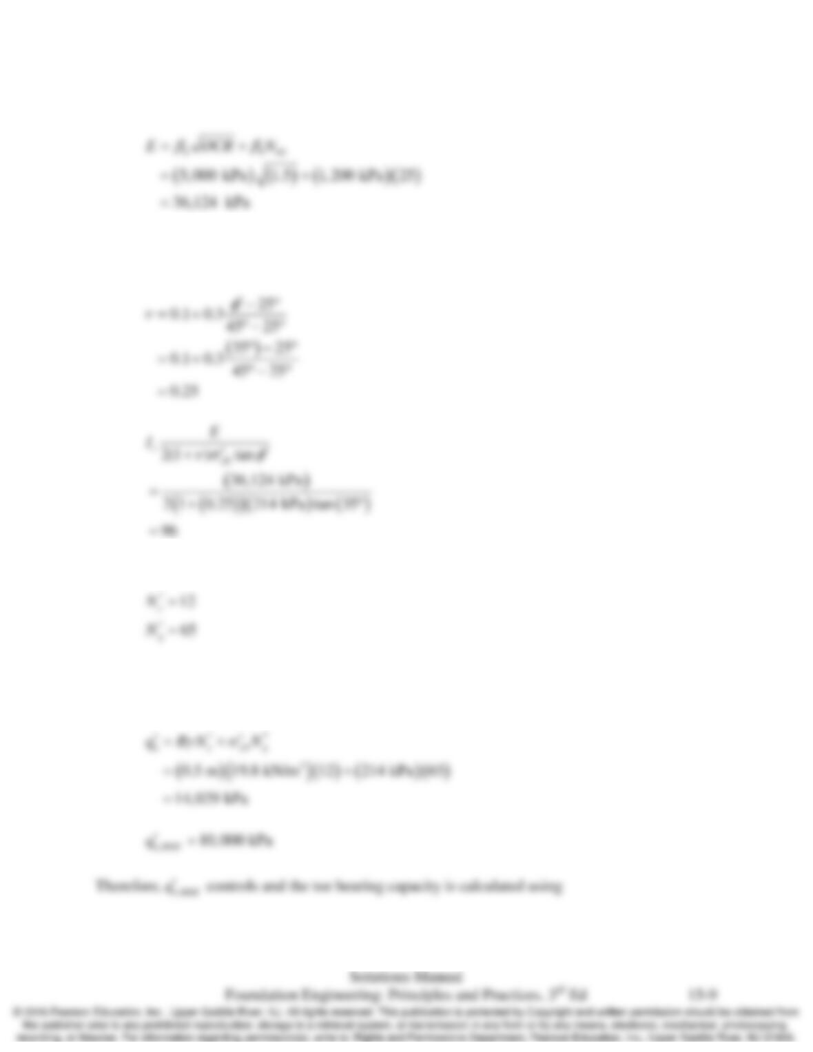
we must first estimate the modulus of elasticity,
E
, of soil within the
zone of influence. One way to do this is to use Equation 4.56 and Table 4.7. Additionally, due to
lacking information we also must estimate the
60
N
value.
Chap.15 Driven Piles: Axial Load Capacity Based on Static Analysis Methods
Now calculate E using Equation 4.56:
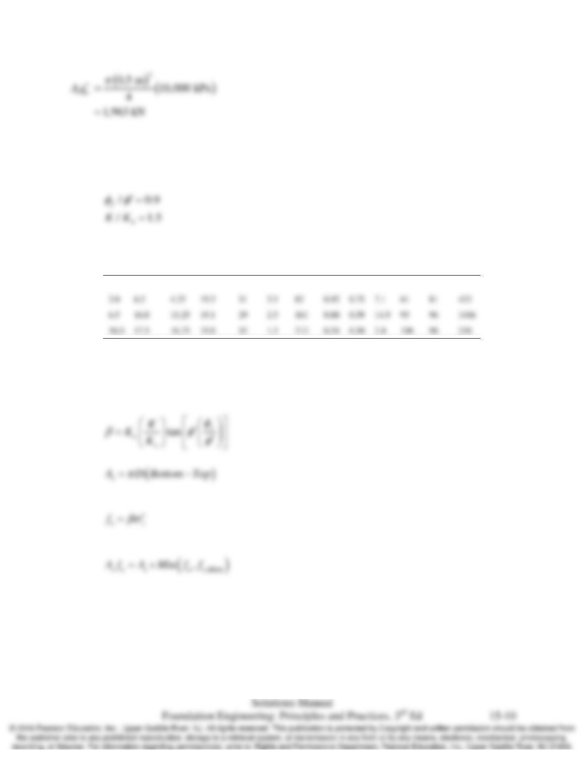
Next we can calculate r
I
. To do this we must first estimate the Poisson’s ratio using Equation
4.44.
Now we can find
*
N
γ
and
*
q
N
using Figures 15.2 and 15.3 respectively.
Next we can substitute into Equation 15.1 and obtain
n
q′
and find the maximum value of
n
q′
from Table 15.1
Chap.15 Driven Piles: Axial Load Capacity Based on Static Analysis Methods
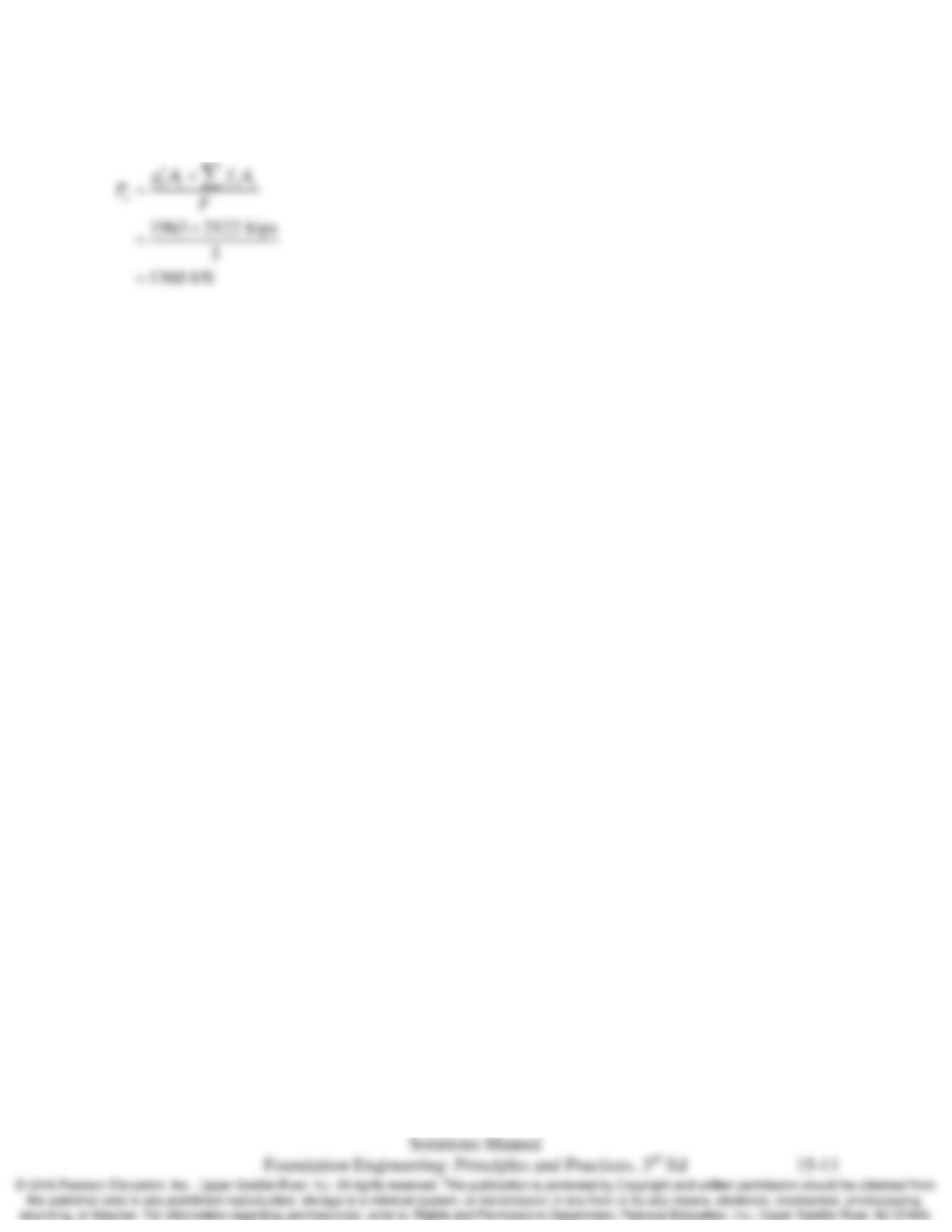
(b) Side Friction
The first step is to determine values for
/
f
φφ
′
and
0
/KK
from Tables 15.2 and 15.3
respectively.
Top
(m)
Bottom
(m)
z
(m)
γ
(kN/m3)
φ
‘
(deg) OCR
σz‘
(kPa) K0 β
As
(m2)
fn
(kPa)
fn, Max
(kPa)
fnAs
(kN)
0.0 2.0 1.00 19.0 28 4.5 19 1.07 0.76 3.1 14 67 43
2122
sin
(1 sin )OCRK
φ
φ
′
′
= −
Chap.15 Driven Piles: Axial Load Capacity Based on Static Analysis Methods
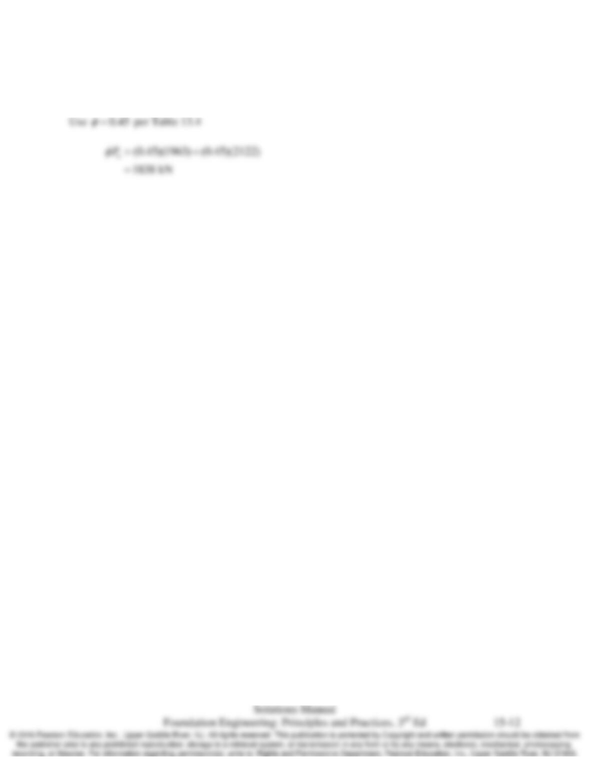
(c) Determine
a
P
Chap.15 Driven Piles: Axial Load Capacity Based on Static Analysis Methods
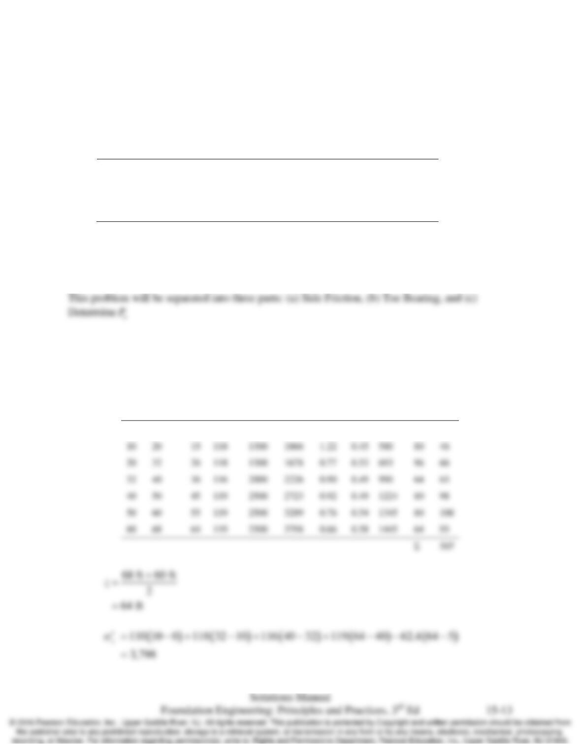
15.6 Using the data in Problem 15.5 and the AASHTO resistance factors, compute
n
P
φ
.
Solution
Chap.15 Driven Piles: Axial Load Capacity Based on Static Analysis Methods
15.7 A 24 inch square prestressed concrete pile is to be driven to a depth of 68 ft into the following
soil profile:
Depth (ft) Soil Classification
Unit Weight,
γ
(lb/ft3)
Undrained Shear
Strength,
u
s
(lb/ft2)
0–10 Silty clay 110 1000
10–32 Clayey silt 118 1300
32–40 Clay 116 2000
40–70 Clay 119 2500
The groundwater table is at a depth of 5 ft. Using the Randolph and Murphy method with a
factor of safety of 3.0, compute the ASD allowable downward load capacity,
a
P
.
Solution
(a) Side Friction
The first step is to produce the following table. Sample calculations are shown below for the last
row in the table.
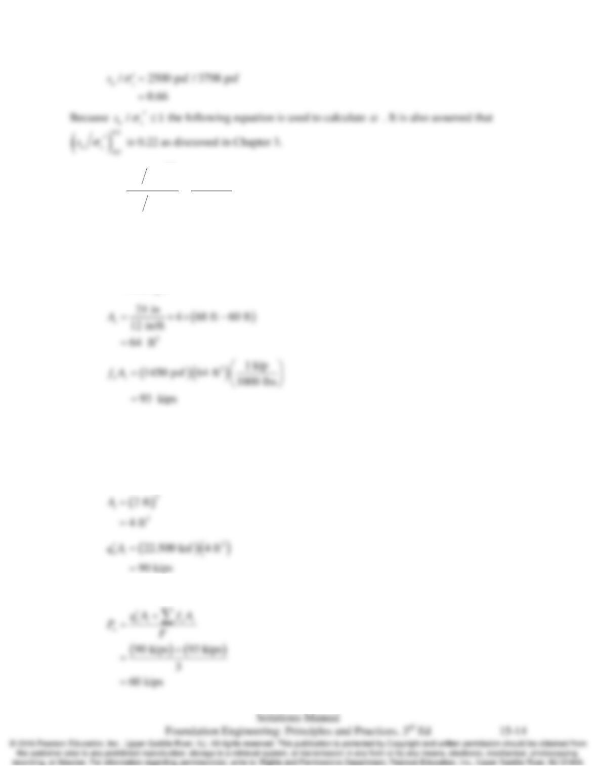
Top Bottom z γ su σzʹ
su/ σzʹ α
fn As fnAs
(ft) (ft) (ft) (lb/ft3) (lb/ft2) (lb/ft2) (lb/ft2) (ft2) (k)
0 10 5 110 1000 550 1.82 0.40 404 80 32
a
Chap.15 Driven Piles: Axial Load Capacity Based on Static Analysis Methods
()
()
( )
( )
0.5
0.5
0.5 0.5
0.22
= 0.66
0.58
uz
NC
uz
s
s
σ
α
σ
′
=′
=
( )( )
0.58 2500 psf
1450 psf
nu
fs
α
=
=
=
(b) Toe Bearing
( )
9
9 2500 psf
22,500 psf
nu
qs
′=
=
=
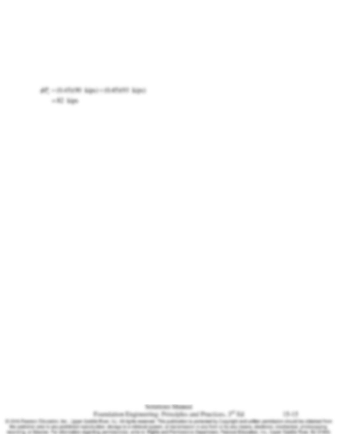
(c) Determine
a
P
Chap.15 Driven Piles: Axial Load Capacity Based on Static Analysis Methods
15.8 Using the data in Problem 15.7 and the AASHTO resistance factors, compute
n
P
φ
.
Solution
Use
0.45
φ
=
per Table 13.4
Chap.15 Driven Piles: Axial Load Capacity Based on Static Analysis Methods
15.9 A 600 mm square prestressed concrete pile is to be driven to a depth of 20.0 m into the following
soil profile:
Depth (m) Soil Classification
Unit Weight,
γ
(kN/m3)
Undrained Shear
Strength,
u
s
(kPa)
0–3.0 Silty clay 17.0 50
3.0–10.2 Clayey silt 17.5 55
10.2–12.0 Clay 17.8 80
12.0–22.0 Clay 18.1 120
The groundwater table is at a depth of 5 ft. Using the Randolph and Murphy method with a
factor of safety of 3.0, compute the ASD allowable downward load capacity,
a
P
.
Solution
(a) Side Friction
The first step is to produce the following table. Sample calculations are shown below for the last
row in the table.
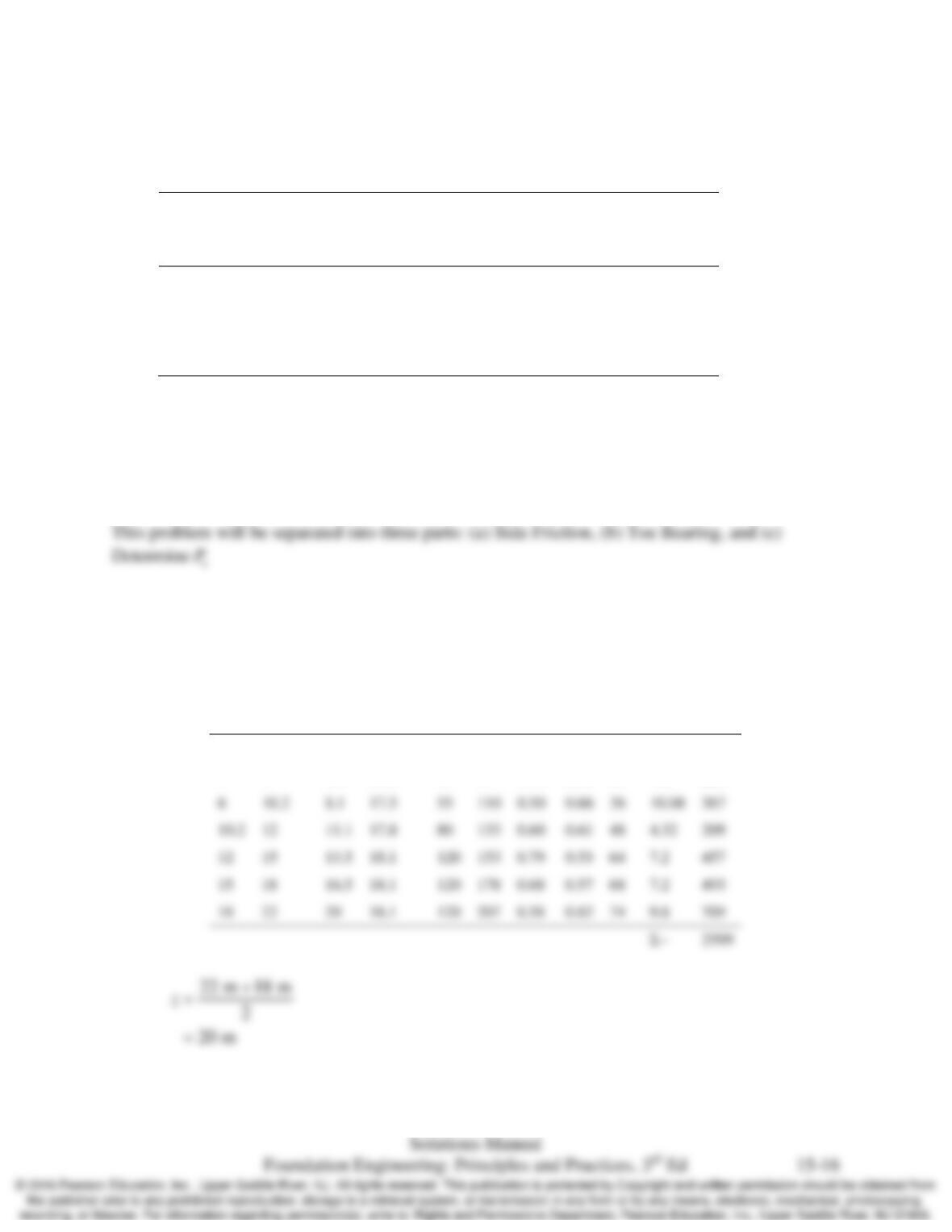
Top Bottom z γ su σzʹ
su/σzʹ α
fn As fnAs
(m) (m) (m) (kN/m3) kPa kpa kPa (m2) (kN)
0 3 1.5 17 50 26 1.96 0.40 20 7.2 143
3 6 4.5 17.5 55 77 0.71 0.56 31 7.2 220
a
Chap.15 Driven Piles: Axial Load Capacity Based on Static Analysis Methods
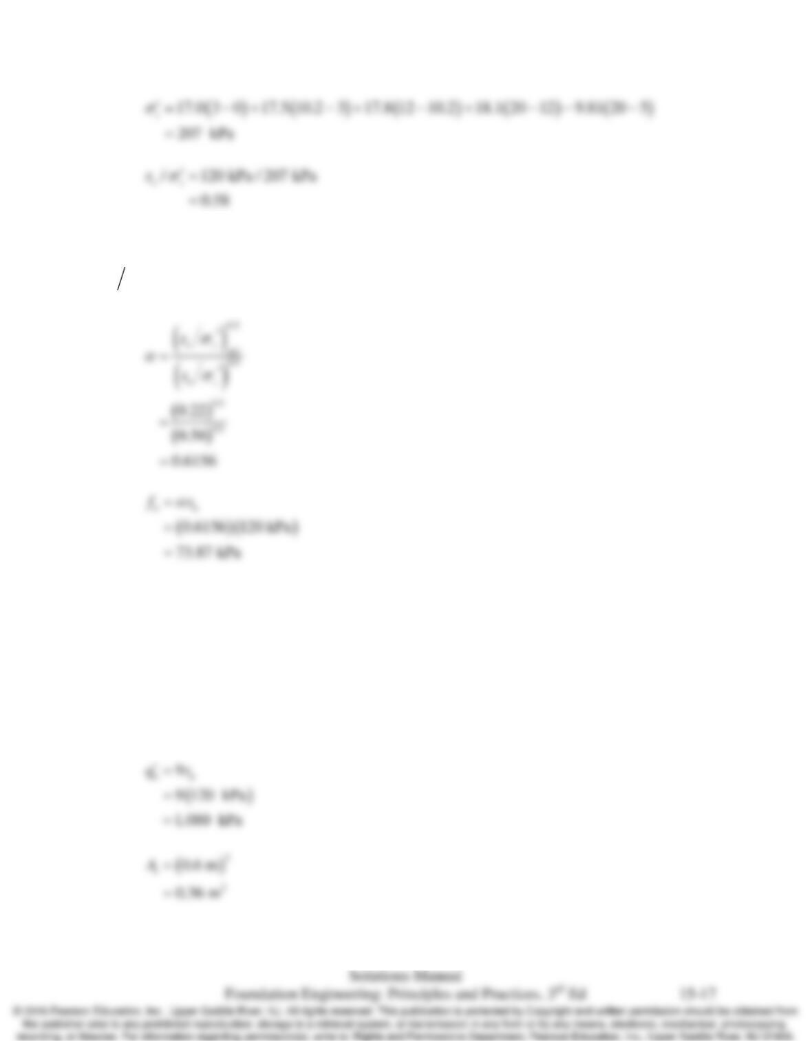
Because
/1
uz
s
σ
′≤
the following equation is used to calculate
α
. It is also assumed that
()
0.5
uz
NC
s
σ
′
is 0.22 as discussed in Chapter 3.
( )
2
0.6 m 4 22 m 18 m
9.6 m
s
A= ×× −
=
( )
( )
2
73.87 kPa 9.6 m
709 kN
ns
fA=
=
(b) Toe Bearing