1
CHAPTER 15
Problem 15.1
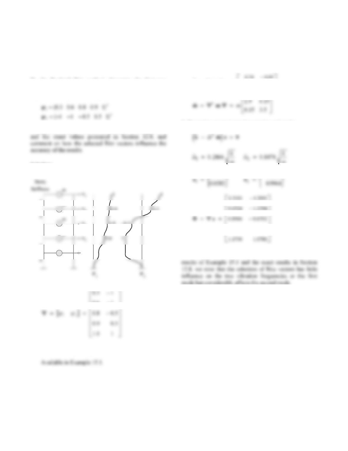
By the Rayleigh–Ritz method, determine the first two
natural vibration frequencies and modes of the system in
Fig. 15.4.1 using the following two Ritz vectors:
Compare these results with those obtained in Example 15.1
Solution:
0.9
0.8
0.3
0.5
– 0.5
– 1
m
u1
k
m
k
k
0.6 1
1. Determine mass and stiffness matrices.
2. Compute
k
and
m.
0.24 0.05
0.05 2.5
Tk
kk
3. Determine approximate frequencies and modes.
m .
m
0 9996
.
0 0853
R
.
1.0428 0.4986
Comparing these
n and n
with the approximate
2
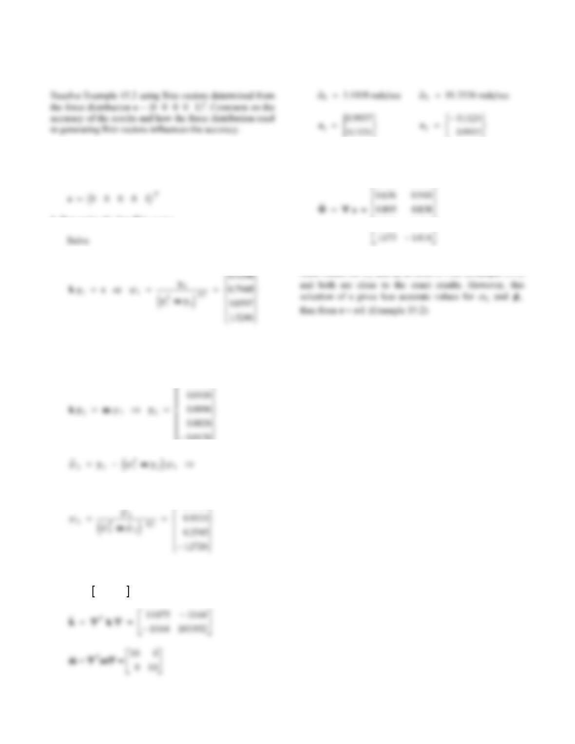
Problem 15.2
Solution:
The k and m are available in Example 15.1 and
1. Determine the first Ritz vector.
0 2649
R
|
U
|
.
2. Determine the second Ritz vector.
Solve
0 0061
0 0130
R
T
|
U
W
|
.
.
0 5939
0 9757
R
|
U
|
.
.
3. Compute
k
and
m.
12
4. Solve ~~~
kmz0
2
ej
.
TU
W
TU
W
5. Compute natural vibration modes.
..
..
L
M
M
O
P
P
0330 0560
1082 0134
We note that this selection of s gives essentially the
same values for
3
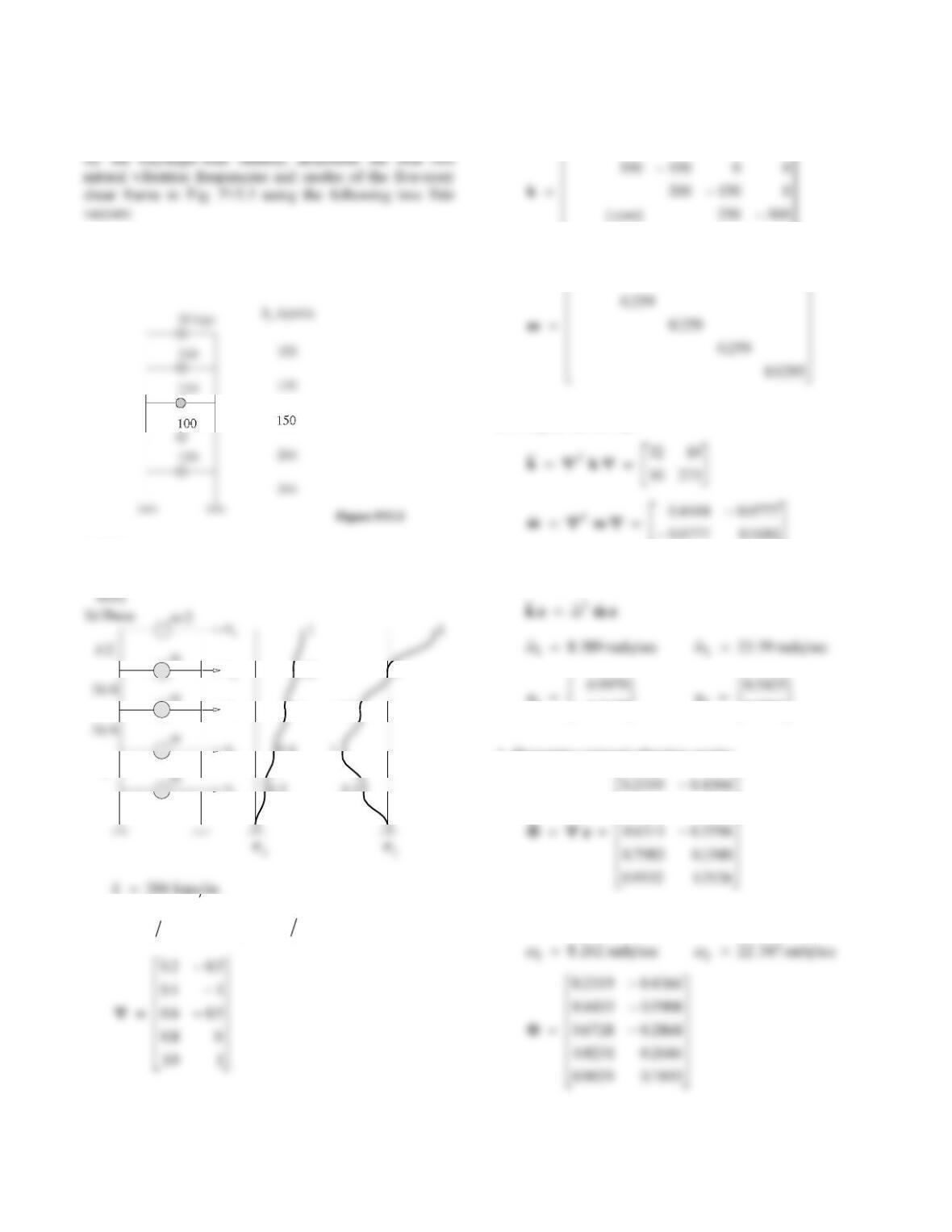
Problem 15.3
1
2
0.2 0.4 0.6 0.8 1
0.5 1 0.5 0 1
T
T
L
N
L
Solution:
0.8
0.6
0.4
0.2
0
– 0.5
– 1
– 0.5
u3
u4
k
m
m
k
in.sec–kip259.0386100 2
m
1. Determine mass and stiffness matrices.
L
N
M
M
O
Q
P
P
400 200 0 0 0
100
L
O
0259
.
2. Compute
k
and
m.
..
N
Q
0 0777 0 5181
3. Solve eigenvalue problem.
00647
S
TU
V
W
. z2
09702
S
TU
V
W
.
4. Determine natural vibration modes.
..
M
M
P
P
0 4639 0 8732
5. Compare with exact values.
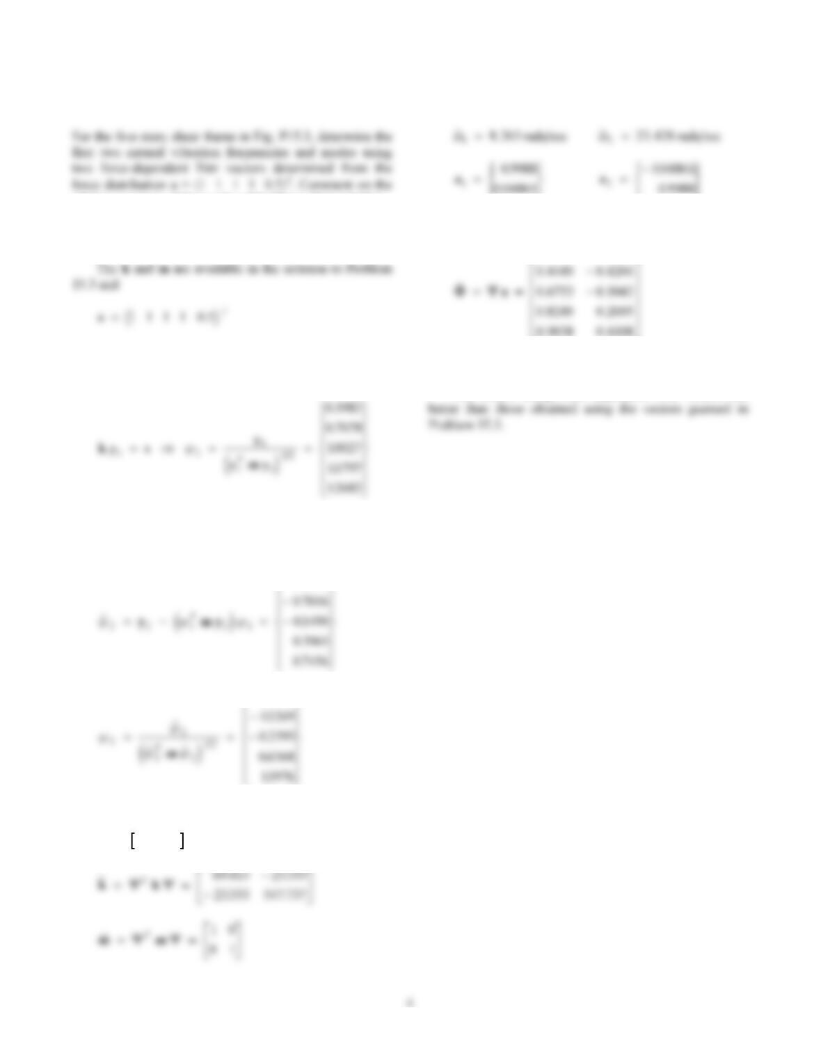
Problem 15.4
relative accuracy of the results of Problems 15.3 and 15.4.
Solution:
1. Determine the first Ritz vector.
Solve
2. Determine the second Ritz vector.
Solve ky m y
212
.
0 7396
R
U
11879
R
T
U
W
.
3. Compute
k
and
m.
12
4. Solve ~~~
kmz0
2
ej
.
TU
W
TU
W
5. Compute natural vibration modes.
0.2319 0.4366
6. Comment on accuracy.
The results using force dependent Ritz vectors are
5
Problem 15.5
Solve Problem 15.4 using the force distribution
s = 0 0 0 0 1T. Comment on the relative accuracy of
the solutions of Problems 15.4 and 15.5.
Solution:
00001
T
s
y10 0050 0 0100 0 0167 0 0233 0 0333…..
T
2. Determine the second Ritz vector,
Orthogonalize y2 with respect to
1:
normalized vector:
3. Compute
~
k
and
~
m.
4. Solve the reduced eigenvalue problem, Eq. (15.3.11).
0 9856
.
01692
.
5. Determine the natural modes, nn
z
, n = 1, 2.
6. Compare with exact results:
10.3407 0.6513 0.9886 1.2093 1.3266 T
from Problems 15.4 and 15.5 are similarly accurate,
whereas the use of
T
5.01111s in Problem
6
Problem 15.6
Solve Problem 15.4 using the force distribution
Solution:
1. Determine the first Ritz vector,
1.
2. Determine the second Ritz vector,
2.
Orthogonalize y2 with respect to
1:
3. Compute
~
k
and
~
m.
12
5. Determine the natural modes, nn
z
, n = 1, 2.
6. Compare with exact results.
10.3407 0.6513 0.9886 1.2093 1.3266 T
7
Problem 15.7
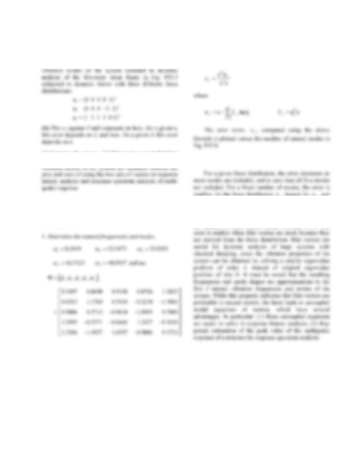
Compute the error eJ where J is the number of Ritz vectors
included in dynamic analysis of the five-story shear frame
Plot eJ against J and comment on how, for a given s, this
error depends on J, and how, for a given J, this error
depends on s.
The stiffness and mass matrices , k and m, are given
12345
0 2534 0 4967 0 8386 0 9932 1 3636
... ..
For the force distribution sb:
12345
0 3052 0 2068 0 3007 1 2005 1 4807
..…
For the force distribution sc:
2122.0796.02697.11878.13981.0
2. Compute eJ.
The error norm, eJ, is defined as:
3. Comments.
The error norm, eJ, computed using the above
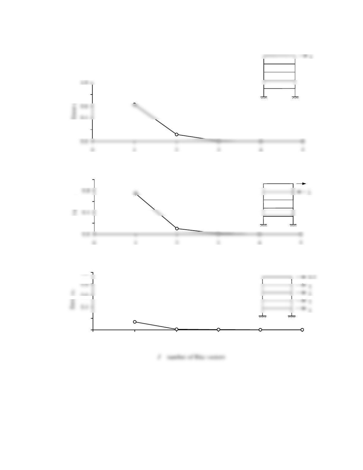
8
0.2
0.8
0.2
0.6
1.0
0.0
0.2
0.6
1.0
012345
Figure P15.7
e
J
1
9
Problem 15.8
(a) Compute the error eJ where J is the number of natural
(c) Compare the error eJ if J Ritz vectors are included in
the analysis (Problem 15.7) versus the error eJ if J natural
Solution:
The stiffness and mass matrices, k and m, are given
in Problem 15.3.
2. Compute eJ.
The error eJ is defined as:
3. Comments.
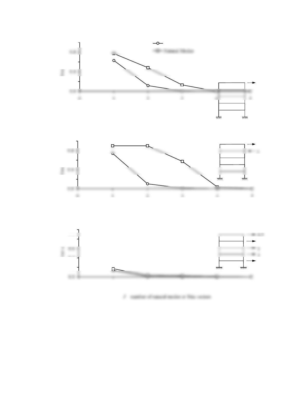
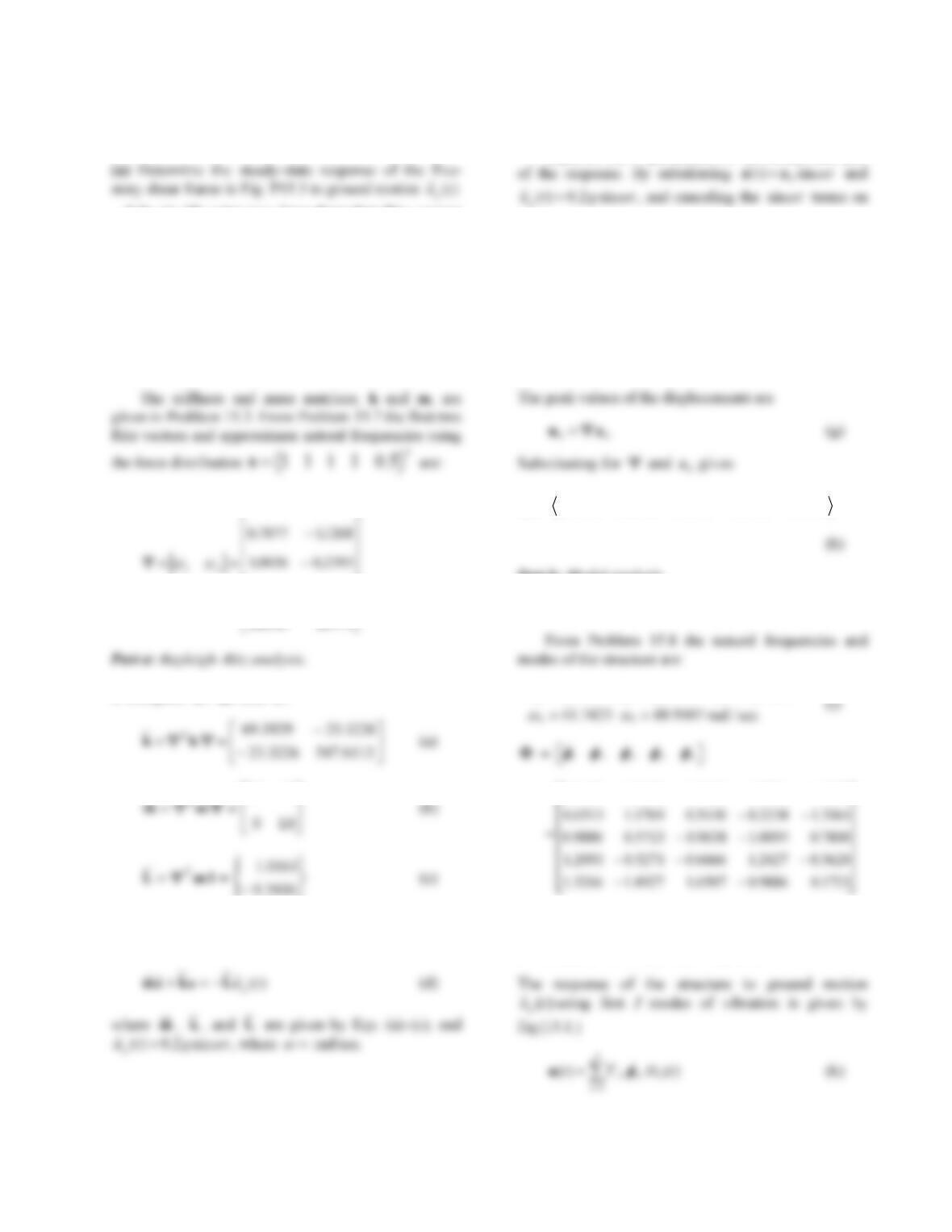
smallest for the force distribution sc, largest for sb, and
has an intermediate value for sa.
Figure P15.8 also shows the error norm, eJ, versus
the number of Ritz vectors (from Problem 15.7). The
10
0.2
0.6
1.0
Ritz vectors
0.2
0.6
1.0
0.2
0.4
0.8
1.0
012345
Figure P15.8
Error eJ
1
1
1
1
11
Problem 15.9
= 0.2g sin 15t using two force-dependent Ritz vectors
determined from the force distribution
s = 1 1 1 1 0.5T. Neglect damping.
(b) Compare these results with those from modal
analysis, including (i) the first two natural vibration
modes, and (ii) all five modes.
Solution:
0 3981 11878
11796 0 6367
1 2680 11974
..
..
..
1. Compute,
k
~,
~
m, and L
~.
2. Set up equations in generalized coordinates; Eq.
(15.3.3) is specialized for this problem.
3. Determine steady-state response.
Equation (d) is specialized for the steady-state part
both sides:
2
0
k15 z 0.2L
g
m
(e)
Solving the two coupled algebraic equations gives
1169.0
4866.0
0
z (f)
T
7570.06484.04599.02126.00548.0
0u
Part b: Modal analysis.
4. Determine frequencies and modes.
8.2619 22.3473 32.9203
1832.18706.09108.08698.03407.0
(j)
5. Determine the steady-state response.
12
where
and )(tDn is governed by
The steady state solution is
Substituting n
and m into Eq. ( l ) gives
Substituting n
from Eq. (o), n
from Eq. (j) and
)(tDn from Eq. (n) into Eq. (k) gives the displace-ment
response:
where 0
u is given as follows. Considering two modes
only, i.e., J2:
(q)
Considering all five modes, i.e., J5:
(r)
6. Comments.
Comparison of Eqs. (h) and (q) with the exact
Percentage Error
u5 –2.7 % 2.6 %
u2 5.0 % 1.2 %