Chap. 14 Piles: Axial Load Capacity Based on Static Load Tests
14.1 A typical deep foundation project may include several hundred piles, but only one or two static
load tests. Thus, the information gained from these test pile must be projected to the production
piles. Describe some of the factors that might cause the load capacity of the production piles to
be different from that of the test pile.
Solution
• Proximity of the tested pile to the actual piles
Chap. 14 Piles: Axial Load Capacity Based on Static Load Tests
14.2 Assume the curve shown in Figure 14.14 has been obtained from a static load test on a 40–ft long,
12-inch square solid concrete pile. Using Davisson’s method, compute the nominal downward
axial load capacity.
Solution
Because Figure 14.14 is in metric units the dimensions must be converted.
Next the cross–sectional area is calculated
A (304.8 mm) 92903 mm= =
Then the and Young’s Modulus is calculated
Chap. 14 Piles: Axial Load Capacity Based on Static Load Tests
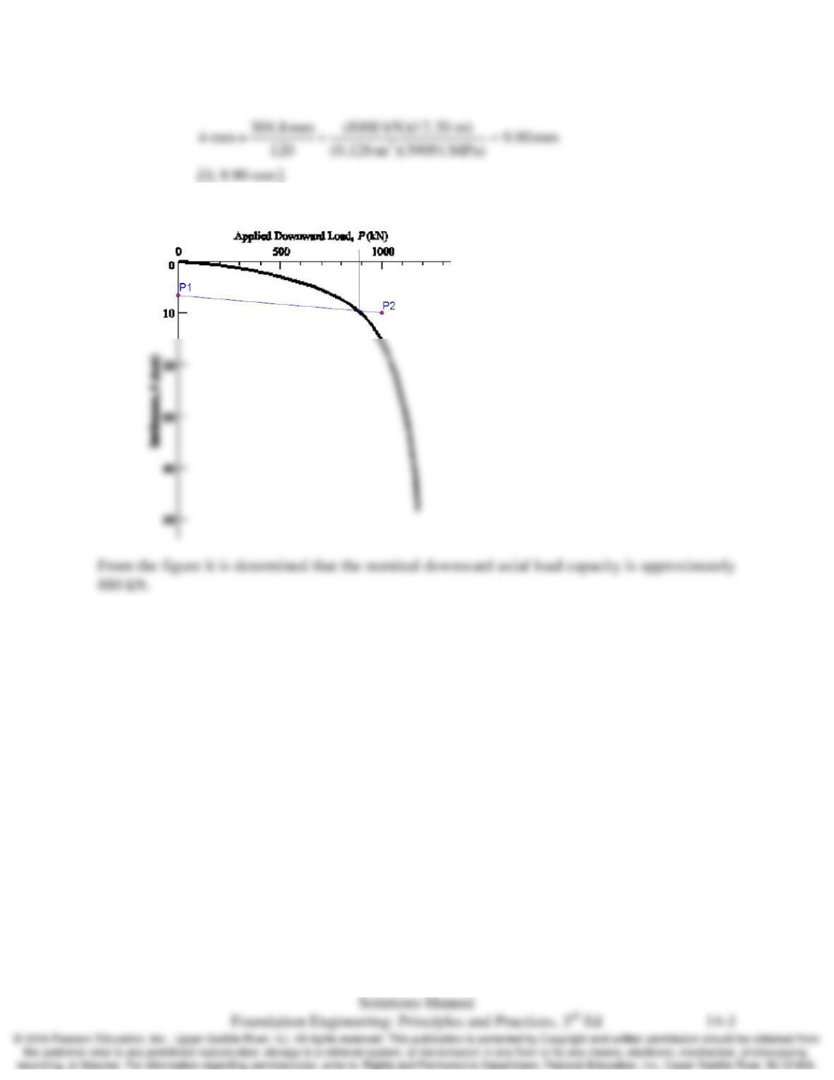
Next, we draw the line connecting points 1 and 2 and find the intersection with the static load
test curve and determine the corresponding nominal downward axial load capacity.
Chap. 14 Piles: Axial Load Capacity Based on Static Load Tests
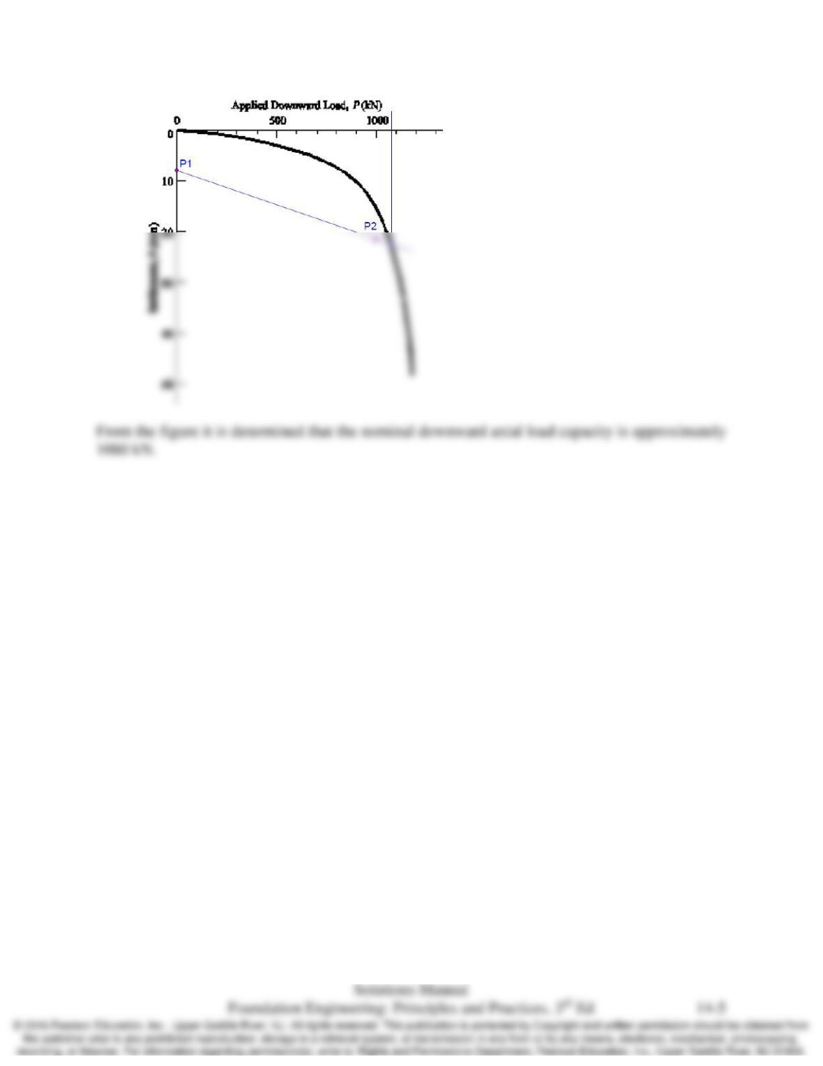
14.3 Assume the curve shown in Figure 14.14 has been obtained from a static load test on a 60 ft long,
PP18x0.375 pile. Using Davisson’s method, compute the nominal downward axial load capacity.
Solution
Because Figure 14.14 is in metric units the dimensions must be converted and the typical metric
Young’s Modulus is assumed.
Then the Cross–Sectional Area is calculated
Chap. 14 Piles: Axial Load Capacity Based on Static Load Tests

Chap. 14 Piles: Axial Load Capacity Based on Static Load Tests
14.4 Solve Problem 14.3 using the Brinch Hansen 80% and 90% methods.
Solution
Chap. 14 Piles: Axial Load Capacity Based on Static Load Tests
14.5 The results of pile load tests are usually considered to be the “correct” load capacity, and all
other analysis methods are compared to this standard. However, there are many ways to conduct
load tests, and many ways to interpret them. Therefore, can we truly establish a single “correct”
capacity for a pile? Explain.
Solution
It is impossible to determine a single “correct” value because there are simply too many
Chap. 14 Piles: Axial Load Capacity Based on Static Load Tests
14.6 A 250–mm square, 15–m long prestressed concrete pile ( fcʹ =40 MPa) was driven at a site in
Amsterdam as described by Heijnen and Janse (1985). A conventional load test conducted 31
days later produced the load–settlement curve shown in Figure 14.14. Using Davisson’s method,
compute the nominal axial downward load capacity of this pile.
Solution
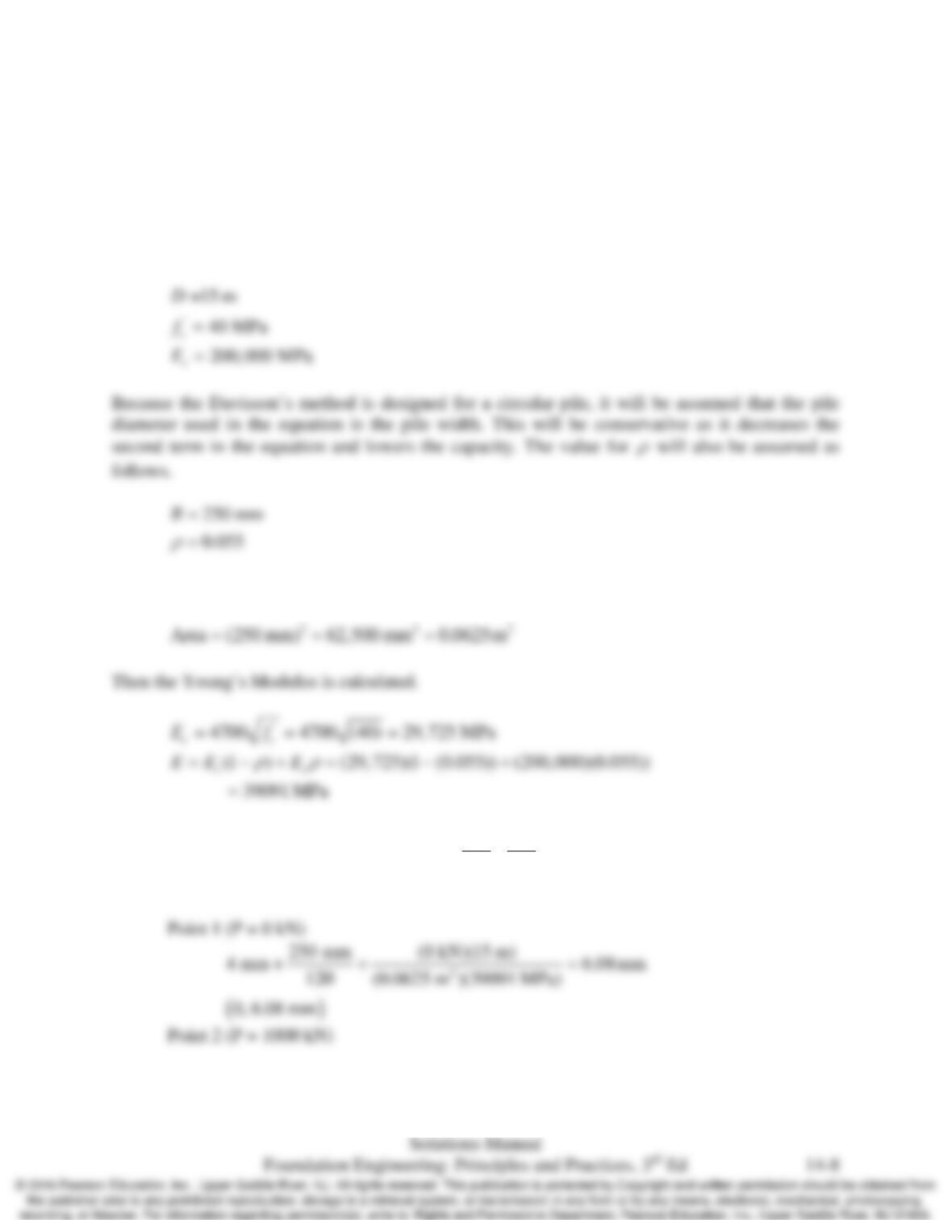
The following information is given by the problem statement
Next the cross–sectional area is calculated
Now we can use Davisson’s formula,
4 mm 120
B PD
AE
++
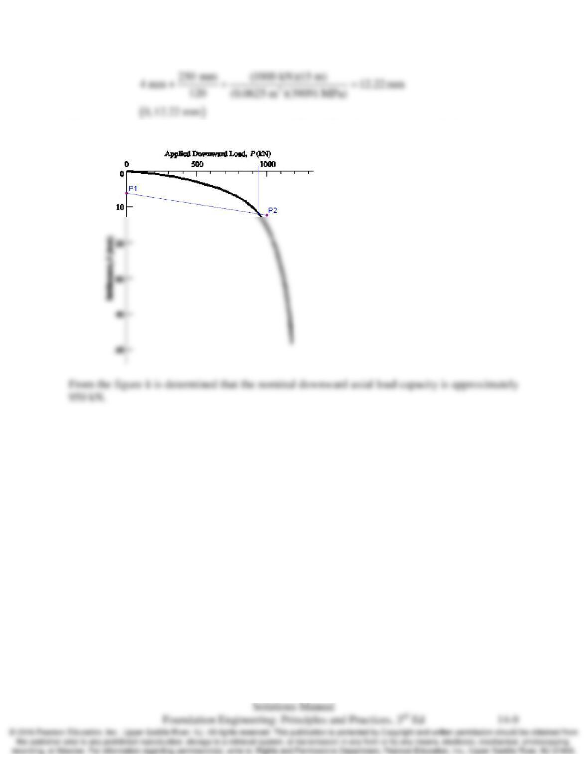
, to calculate two points with different
assumed values for P to plot on Figure 14.14
Chap. 14 Piles: Axial Load Capacity Based on Static Load Tests
Next, we draw the line connecting points 1 and 2 and find the intersection with the static load
test curve and determine the corresponding nominal downward axial load capacity.
Chap. 14 Piles: Axial Load Capacity Based on Static Load Tests
14.7 Solve Problem 14.6 using the Brinch Hansen 80% and 90% methods.
Solution
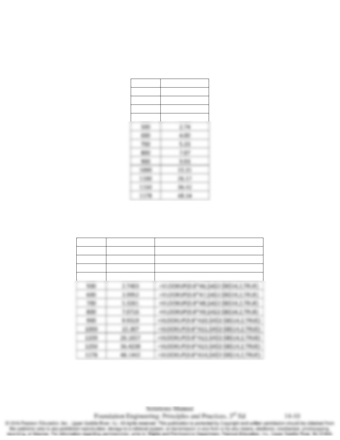
The first step is to interpret Figure 14.14 and determine a series of points to be used in an Excel
analysis. Choosing more points will make the analysis more accurate. One interpretation is:
Load (kN)
Settlement (mm)
0
0.00
200
0.48
300
1.11
400
1.92
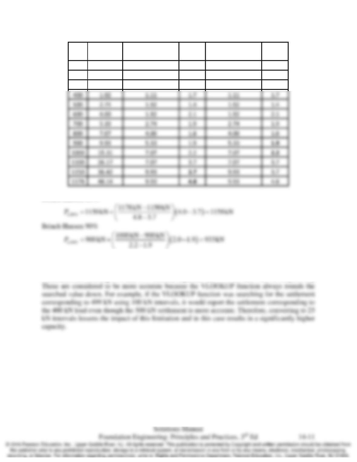
The next step uses the excel VLOOKUP function to determine the settlements corresponding to
0.80Pn and 0.90Pn to simplify calculations. The formulas for 0.80Pn are as follows where A1 is
the “Load (kN)” Cell.
Load (kN)
Settlement (mm)
80%*Displacement (mm)
0
0
=VLOOKUP(0.8*A2,$A$2:$B$14,2,TRUE)
200
0.4751
=VLOOKUP(0.8*A3,$A$2:$B$14,2,TRUE)
300
1.1060
=VLOOKUP(0.8*A4,$A$2:$B$14,2,TRUE)
400
1.9181
=VLOOKUP(0.8*A5,$A$2:$B$14,2,TRUE)
500
600
3.9952
=VLOOKUP(0.8*A7,$A$2:$B$14,2,TRUE)
700
5.3261
=VLOOKUP(0.8*A8,$A$2:$B$14,2,TRUE)
800
7.0716
=VLOOKUP(0.8*A9,$A$2:$B$14,2,TRUE)
900
9.9319
15.307
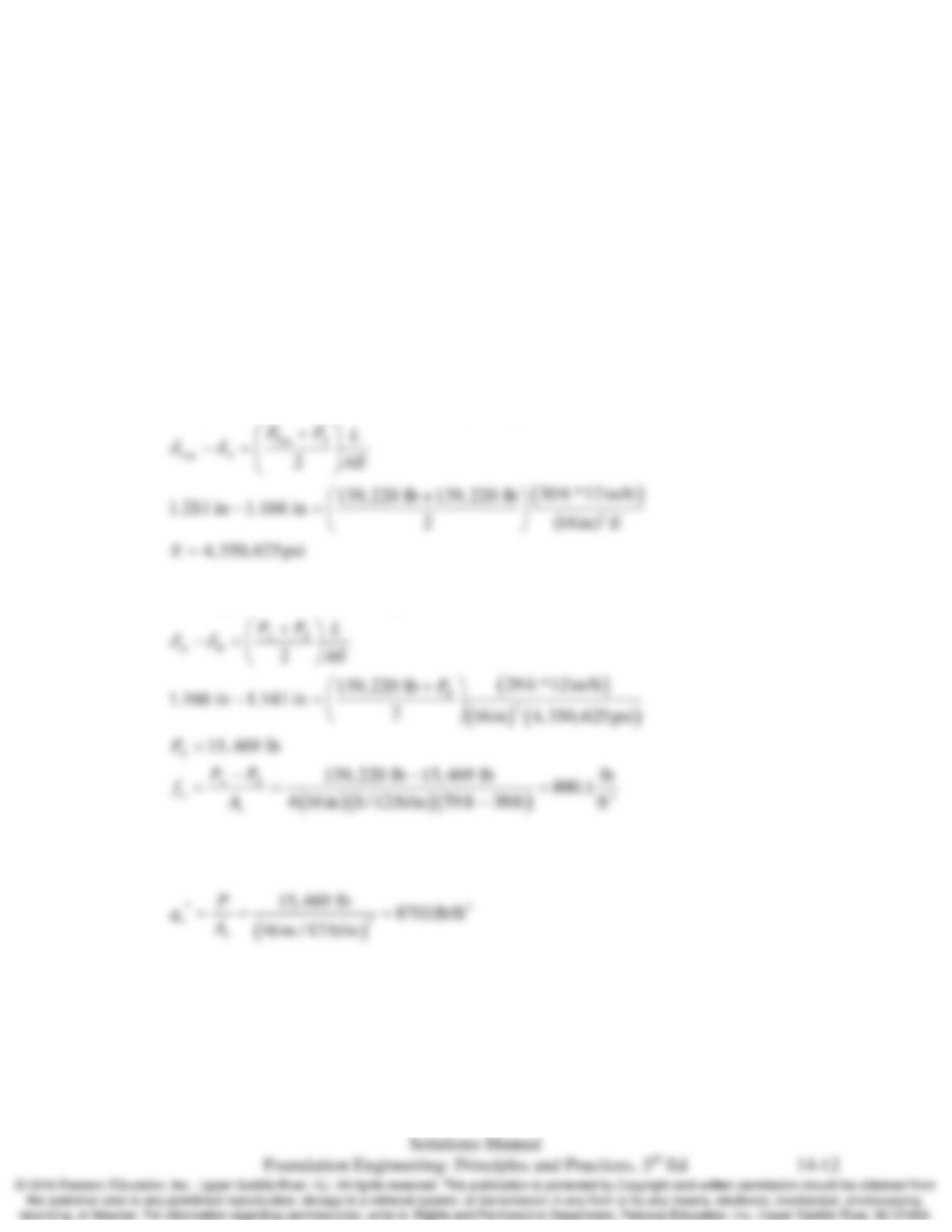
The settlement ratios are then calculated and the Pn corresponding to a ratio of 4 and 2 for 80%
90% displacements respectively are determined by interpellation.
500
2.74
600
4.00
700
5.33
800
7.07
900
9.93
Chap. 14 Piles: Axial Load Capacity Based on Static Load Tests
Load
(kN)
Settlement
(mm)
80%*Displacement
(mm)
80%
Ratio
90%*Displacement
(mm)
90%
Ratio
0
0.00
0.00
#DIV/0!
0.00
#DIV/0!
200
0.48
0.00
#DIV/0!
0.00
#DIV/0!
300
1.11
0.48
2.3
0.48
2.3
Brinch Hansen 80%:
Note:
If the 100 kN intervals are changed to intervals of 25kN by interpolating the loads and
settlements the resulting 80% and 90% nominal capacities are 1171 kN and 1125 kN respectively.
400
1.92
1.11
1.7
1.11
1.7
500
2.74
1.92
1.4
1.92
1.4
600
4.00
1.92
2.1
1.92
2.1
700
5.33
2.74
1.9
2.74
1.9
800
7.07
4.00
1.8
4.00
1.8
900
9.93
5.33
1.9
5.33
7.07
2.2
7.07
7.07
3.7
7.07
3.7
9.93
9.93
3.7
9.93
9.93
4.8
Chap. 14 Piles: Axial Load Capacity Based on Static Load Tests
14.8 A static load test has been conducted on a 60–ft long, 16–inch square reinforced concrete pile
which has been driven from a barge through 20 ft of water, then 31 ft into the underlying soil.
Telltale rods A and B have been embedded at points 30 ft and 59 ft from the top of the pile,
respectively. The data recorded at failure was as follows: Load at head = 139,220 lb, settlement
at head = 1.211 in, settlement of tell-tale rod A = 1.166 in, settlement of tell-tale rod B = 1.141 in.
Use the data from tell–tale rod A to compute the modulus of elasticity of the pile, then use this
value and the remaining data to compute
n
q′
and the average
n
f
value.
Hint: Tell–tale rod A is anchored only 1 ft from the mud line (the top of the soil). There is
essentially no side–friction resistance between the top of the pile and this point, so the force at a
depth of 30 ft is essentially the same as that at the top of the pile.
Solution
The first step is to compute modulus of elasticity using the data from telltale rods at 0 and 30 ft.
Next the average
n
f
is computed using the data from telltale rods A and B.
Lastly,
n
q′
is calculated assuming the last foot of side friction is negligible.
14.9 An Osterberg load test is to be conducted on a 60 inch diameter, 75 ft long drilled shaft. The
expected nominal side friction capacity is 2000 lb/ft2 and the expected nominal net toe bearing
capacity is 60,000 lb/ft2. a) Determine the optimal jack location such that the load capacity
above the jack is equal to that below the jack. b) Compute the required jack capacity.
Solution
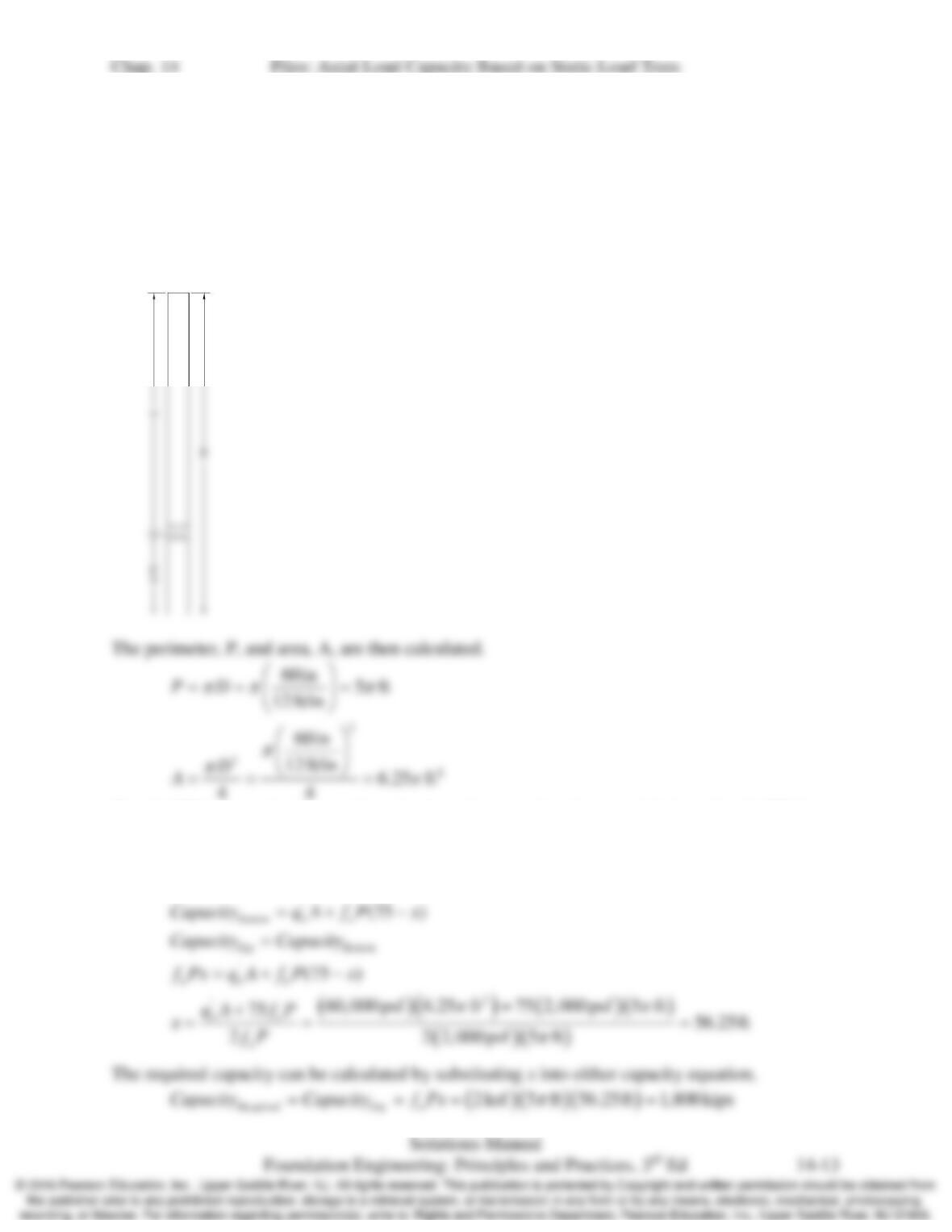
The first step is to define the distance to the O–CELL. This solution assumes it is the distance
from the top of the pile as indicated.
The O–CELL is optimally positioned when the capacity above and below the O–CELL are
identical. Therefore, the top and bottom capacities are determined in terms of x and then equated
to solve for x.
Top n
Capacity f Px
=